Machine Learning with tidymodels – Part 2

Bagged trees, random forests, and boosted trees

Published

Jan 27, 2025

In the previous post, we focused on some fundamental steps involved in machine learning exercises: data splitting and resampling, preprocessing and model specification, creating workflows and workflow sets, and training them. We saw that we could use rsample, recipes, parsnip, workflows, and workflowsets packages bundled in tidymodels to implement these steps in R easily. In this post, we will concentrate on tree-based models, a nonlinear model family, to illustrate how to tune model hyperparameters using tidymodels’ tune and dials packages.

We will use the same code from the previous post to create the training and test sets and cross-validation resamples.

library(tidymodels)
tidymodels_prefer()

data(ames)
ames = mutate(ames, Sale_Price = log10(Sale_Price))

set.seed(2025)
ames_split = initial_split(ames, prop = 0.8, strata = Sale_Price)
ames_train = training(ames_split)
ames_test = testing(ames_split)

set.seed(342)
ames_folds = vfold_cv(ames_train, strata = Sale_Price) # 10-fold single-repeat CV

Decision trees

Key concepts

Tree-based models partition or stratify the feature space by using simple splitting rules to create groups or regions of observations. These methods then use the same average response value in a given group to predict a response value for all the observations assigned to that group. Below, we see a visual representation of the splitting rules generated by a tree-based model trained on the Ames housing data. Since splitting rules can be represented as an upside-down tree, tree-based models are known as decision trees.

Code

library(rpart)
library(rpart.plot)

par(bg="#99badd")
rpart(Sale_Price  ~ ., ames_train, method = "anova") |>
  rpart.plot(
    faclen = 1, box.palette = "Oranges", Margin = -0.06, 
    main = "Pruned decision tree for the Ames housing data", 
    yes.text = "YES", no.text = "NO"
  )

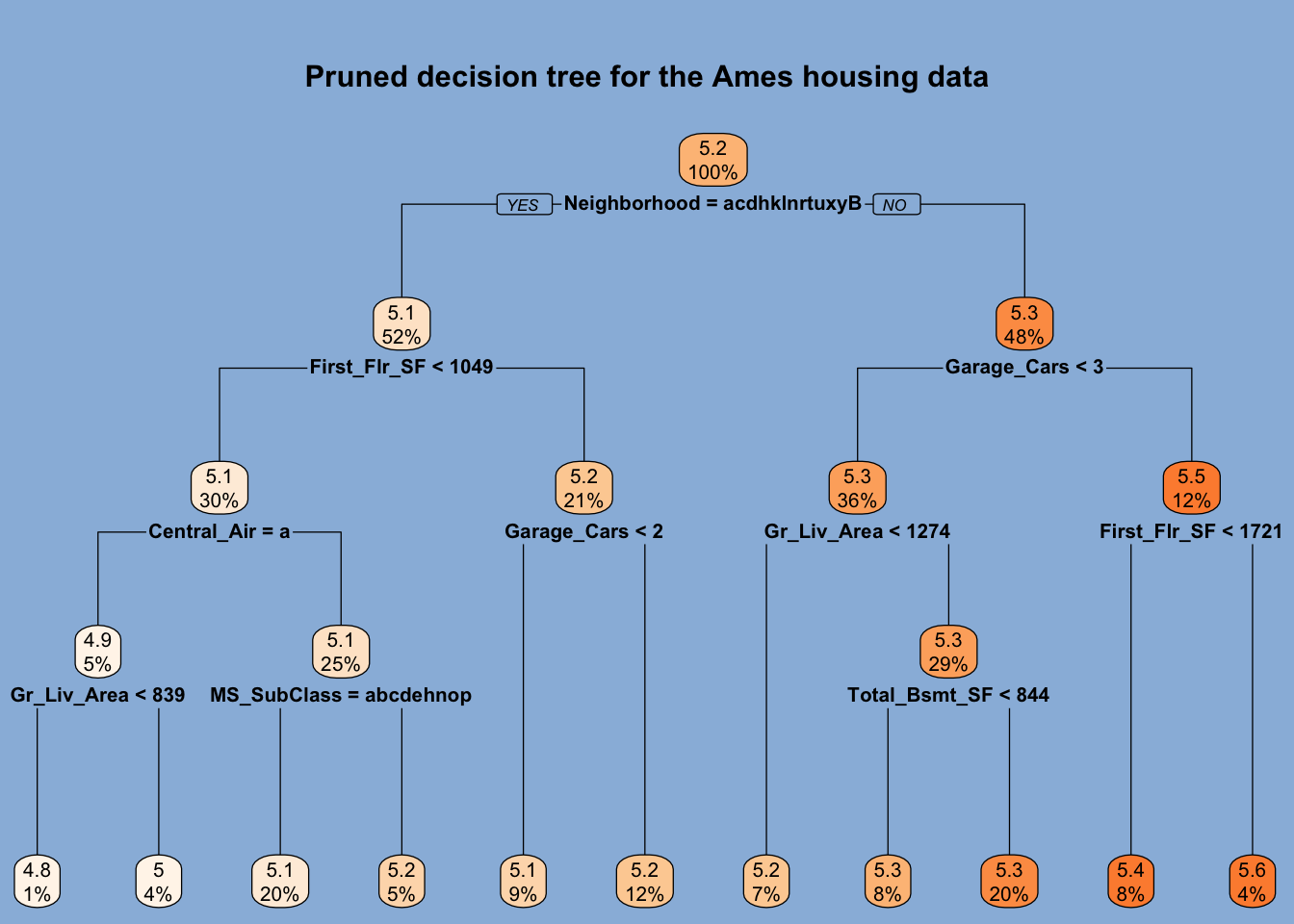
Decision trees use binary splitting rules to partition the feature space. In the case of numerical variables, any given observation may or may not be lower than the split value. Those lower than the split value are placed in the left branch, and those equal to or greater than the split value are placed in the right branch. For categorical variables, any given observation may belong to a specific collection of categories or not. Those that do are placed in the left branch and those that do not are placed in the right branch. Branches are represented by the vertical lines that are attached to nodes. The node at the top is called the root node and contains all training data. The nodes at the bottom that are not further split are called terminal nodes or leaves. All other nodes are called internal nodes. Note that the number of terminal nodes is simply one greater than the number of splits. In the tree above, there are 10 splits and 11 terminal nodes.

We see that the model used the Neighborhood feature for the first split. Those homes not located in those 13 neighborhoods whose names are represented by a distinct letter below the root node are placed in the right branch.¹ These homes make up 48% of all, and their average sale price is $10^{5.3} = 199, 526$ dollars. These homes are then further split using the “Garage_Car (the number of cars the garage can accommodate) is less than 3” rule, and those that meet the rule, 36% of all, are placed in the left branch. These homes are further split using the “Gr_Liv_Area (above-ground living area) is less than 1274 square feet” rule, and those that meet the rule are placed in the left node. So the model computes the average price for the homes that are not located in those 13 neighborhoods with smaller than 3-car garages and with less than 1274 sq ft above-ground living area, 7% of all, as $10^{5.2} = 158, 489$ dollars. We can use this average price to predict a sale price for similar houses.

Since splitting is binary and repetitive, it is called recursive binary splitting. How does the algorithm decide which variable and split value/level to split? For regression problems, the variable and its split value are chosen such that they reduce the sum of squared errors (SSE) the most, which is defined as follows:

$S S E = \sum_{i \in R_{1}} (y_{i} - r_{1})^{2} + \sum_{i \in R_{2}} (y_{i} - r_{2})^{2}$

where $R_{1}$ and $R_{2}$ represent the left and right branches/regions, and $r_{1}$ and $r_{2}$ are the average response values for those regions, respectively.²

If the algorithm were to keep splitting to achieve the largest reduction in SSE, it would fit a highly complex tree with a relatively large depth and many terminal nodes. By so doing, it could reduce the overall SSE to the minimum. However, we do not necessarily want this to happen because the model would overfit the data. A deep tree with numerous terminal nodes can reduce the training prediction error. Due to their structure based on recursive splitting, decision trees are very good at this. The problem is that using different training data would lead to a different tree and predictions with unseen data. This means that predictions would have a large variance, making them unreliable. This is the unavoidable bias-variance trade-off. A clever workaround is to prevent the tree from getting too deep/complex at the expense of some bias.

One strategy is to use a threshold value as a criterion for splitting. In other words, a node will be split if doing so reduces SSE by at least that threshold value. This value is called the cost complexity parameter. Unlike the coefficients in a linear regression model, this parameter cannot be directly estimated from the training data, and we must determine it. In this sense, the cost complexity parameter is a tuning parameter or hyperparameter. But how should we choose an optimum value for this parameter? This is where resampling comes into play. We can use k-fold cross-validation or the validation set approach to tune the cost complexity hyperparameter. Out of a set of different candidate values, the value that minimizes a given measure of prediction error computed against the analysis set (e.g., RMSE) is picked as the optimum value. This is the central idea in tuning model hyperparameters.

Preventing a tree from growing too complex in the manner outlined above means preventing some splits. The resulting tree would look pruned rather than full-grown. So, we prune a tree using a cost complexity parameter, a strategy known as cost complexity pruning. Two other main parameters that can also be tuned along with cost complexity are the maximum tree depth (or height) and the minimum number of observations required in a node to attempt a split (i.e., minimum node size).

Growing a tree

Let’s review the key concepts in the first post using tidymodels tools to grow the tree above again. Below, we will specify the model, create a workflow, and then fit it to the entire training data. parsnip provides the decision_tree() function to specify the model type as a tree. It can work with different independent functions (i.e., engines) to fit a tree, and it uses rpart() as its default computational engine.³

decision_tree() has two main arguments, tree_depth and min_n, and one engine argument, cost_complexity. The main arguments are common to different engines that can fit a decision tree. The parsnip functions help to streamline the tuning process by providing these arguments. All three arguments are set to NULL by default, and that means that the underlying engine will use its default values for the corresponding arguments.⁴ method is an engine argument and not defined in decision_tree(), so we must pass it to set_engine(). For regression problems, it should be set to “anova”.

tree_spec = 
  decision_tree() |>
  set_engine("rpart", method = "anova") |>
  set_mode("regression")

tree_wflow = 
  workflow() |>
  add_formula(Sale_Price ~ .) |>
  add_model(tree_spec)

tree_fit = fit(tree_wflow, ames_train)

Using extract_fit_engine(), we can extract the fit object from a workflow. The returned fit object prints the splitting rules and node information. In a regression context, deviance refers to SSE.

tree_fit |> extract_fit_engine()
#> n= 2342 
#> 
#> node), split, n, deviance, yval
#>       * denotes terminal node
#> 
#>  1) root 2342 74.7794300 5.220495  
#>    2) Neighborhood=North_Ames,Old_Town,Edwards,Sawyer,Mitchell,Brookside,Iowa_DOT_and_Rail_Road,South_and_West_of_Iowa_State_University,Meadow_Village,Briardale,Northpark_Villa,Blueste,Landmark 1208 21.2373900 5.108366  
#>      4) First_Flr_SF< 1048.5 706 11.5850500 5.060885  
#>        8) Central_Air=N 118  3.9306040 4.929915  
#>         16) Gr_Liv_Area< 838.5 31  1.3770960 4.768087 *
#>         17) Gr_Liv_Area>=838.5 87  1.4523900 4.987578 *
#>        9) Central_Air=Y 588  5.2241910 5.087168  
#>         18) MS_SubClass=One_Story_1946_and_Newer_All_Styles,One_Story_1945_and_Older,One_Story_with_Finished_Attic_All_Ages,One_and_Half_Story_Unfinished_All_Ages,One_and_Half_Story_Finished_All_Ages,Two_and_Half_Story_All_Ages,Two_Story_PUD_1946_and_Newer,PUD_Multilevel_Split_Level_Foyer,Two_Family_conversion_All_Styles_and_Ages 463  3.4437510 5.066266 *
#>         19) MS_SubClass=Two_Story_1946_and_Newer,Two_Story_1945_and_Older,Split_or_Multilevel,Split_Foyer,Duplex_All_Styles_and_Ages,One_Story_PUD_1946_and_Newer 125  0.8288664 5.164591 *
#>      5) First_Flr_SF>=1048.5 502  5.8222100 5.175143  
#>       10) Garage_Cars< 1.5 210  1.7406580 5.125375 *
#>       11) Garage_Cars>=1.5 292  3.1873370 5.210935 *
#>    3) Neighborhood=College_Creek,Somerset,Northridge_Heights,Gilbert,Northwest_Ames,Sawyer_West,Crawford,Timberland,Northridge,Stone_Brook,Clear_Creek,Bloomington_Heights,Veenker,Greens,Green_Hills 1134 22.1750500 5.339940  
#>      6) Garage_Cars< 2.5 852  8.9867470 5.289142  
#>       12) Gr_Liv_Area< 1273.5 174  1.1167970 5.183332 *
#>       13) Gr_Liv_Area>=1273.5 678  5.4219130 5.316297  
#>         26) Total_Bsmt_SF< 843.5 199  0.7469760 5.250873 *
#>         27) Total_Bsmt_SF>=843.5 479  3.4692680 5.343478 *
#>      7) Garage_Cars>=2.5 282  4.3473560 5.493416  
#>       14) First_Flr_SF< 1721 194  1.7771910 5.444104 *
#>       15) First_Flr_SF>=1721 88  1.0584690 5.602125 *

As we pointed out before, this tree is not relatively deep. This is so because rpart() conducts its internal cross-validation to find the best cost complexity value and prunes the tree using that value. Below, we will tune the same parameter ourselves.

Recall that the regression tree algorithm uses the maximum reduction in SSE to determine the feature and its value/level to split a node. The fact that our tree uses the Neighborhood feature first implies that it is potentially the most important variable in reducing the prediction error. One can sum up the reductions in SSE from using a given feature to split nodes to compute the total decrease in SSE for all features. The total reduction in SSE attributed to a feature represents its variable importance (VI) score. VI scores can be turned into an index where the score for the most important variable is assigned to 100. The vip package computes or accesses VI scores for many models using the above and other methods and generates VI plots. VI scores are not simply calculated from a single/best model fit and obtained through cross-validation. Below, we use the vip() function to plot the VI scores for the top 10 features from our decision tree model.⁵ We see that Neighborhood is the most important variable. Interestingly, some features such as Year_Built and Longitude received high VI scores even though they were not picked up in the best fit.

library(vip)
vip(tree_fit, num_features = 10, geom = "point")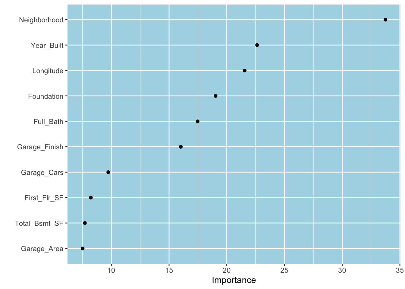

Tuning hyperparameters

Tuning model hyperparameters (or tuning parameters) with tidymodels involves essentially three steps:

Tag tuning parameters to denote which ones are to be tuned. This step consists of setting tuning parameters to tune() in either model specification functions or recipes.
Create a grid, a combination of different values of tuning parameters to be tried out by the primary tuning function, tune_grid()⁶, and
Run tune_grid() to compute performance metrics against the assessment sets for each combination of parameter values.

Return to our model specification function, decision_tree(). Below, we set both cost_complexity and min_n to tune() to tag them for tuning.⁷ Since we will be doing our cross-validation, we set the xval engine argument to zero to tell rpart() not to perform its internal cross-validation.⁸

tree_spec = 
  decision_tree(cost_complexity = tune(), min_n = tune()) |>
  set_engine("rpart", xval = 0) |>
  set_mode("regression")

tree_wflow = 
  workflow() |>
  add_formula(Sale_Price ~ .) |>
  add_model(tree_spec)

Parameter objects

The dials package provides numerous functions to create parameter objects under the hood. These functions are named the same as the tuning parameter on which they operate. For instance, the cost_complexity() function creates a parameter object as a list to store information on the cost complexity parameter, including its default range.

cost_complexity()
#> Cost-Complexity Parameter (quantitative)
#> Transformer: log-10 [1e-100, Inf]
#> Range (transformed scale): [-10, -1]

Note that executing the function prints its transformer function and the range on the transformed scale. The natural/actual range is then $[10^{- 10}, 10^{- 1}] = [10^{- 10}, 0.1]$ .⁹ For some numeric values, it might be more intuitive to set the natural range directly via the range and trans arguments as follows:

cost_complexity(range = c(0.01, 0.1), trans = NULL)
#> Cost-Complexity Parameter (quantitative)
#> Range: [0.01, 0.1]

No transformer function is needed for tuning parameters such as min_n (minimal node size).

min_n()
#> Minimal Node Size (quantitative)
#> Range: [2, 40]

Let’s extract the tuning parameters we tagged in our tree workflow. tidymodels has two functions, extract_parameter_dials() and extract_parameter_set_dials(), to extract the tuning parameters we tag in workflows and workflow sets.¹⁰ extract_parameter_set_dials() returns a parameters object. The object is a list printed as a data frame for convenience. The type column stores the name of the parameter. The identifier column stores the same name unless the tune() function is provided with a character string to use a different parameter name. “nparam” part of the text under the object column indicates that the parameter is numeric, and “[+]” indicates that it was created/finalized. This column is, in fact, a list and stores the same information produced by the cost_complexity() function.¹¹

tree_param = 
  tree_wflow |>
  extract_parameter_set_dials()
tree_param
#> Collection of 2 parameters for tuning
#> 
#>       identifier            type    object
#>  cost_complexity cost_complexity nparam[+]
#>            min_n           min_n nparam[+]

Sometimes, we may need a different range than the default range for a parameter. We can use the update() function in stats to achieve this. Let’s say we want to use the following range for the cost complexity parameter: $[10^{- 5}, 10^{- 1}]$ .¹² We create the parameter object with its corresponding function and pass it into the update() function using the same name it has in the workflow.

tree_param = 
  tree_param |>
  update(cost_complexity = cost_complexity(range = c(-5, -1)))

tree_param$object[[1]]
#> Cost-Complexity Parameter (quantitative)
#> Transformer: log-10 [1e-100, Inf]
#> Range (transformed scale): [-5, -1]

Grids

So far, we have seen how to tag tuning parameters for tuning, what happens under the hood to create the corresponding parameter objects, and how to extract and update these objects. These steps also generate a default range for parameters that we can change. But how do we create a grid containing the specific values with which we want to see how the model performs? This is where the grid_*() functions in the dials package come into play.

Below, we use the grid_regular() function to create five separate values for each parameter in tree_param and then combine them factorially to have 25 points.¹³ Note that the function returns a data frame where each row has a different parameter value combination.

grid_reg = tree_param |> 
  grid_regular(levels = 5)
grid_reg
#> # A tibble: 25 × 2
#>    cost_complexity min_n
#>              <dbl> <int>
#>  1         0.00001     2
#>  2         0.0001      2
#>  3         0.001       2
#>  4         0.01        2
#>  5         0.1         2
#>  6         0.00001    11
#>  7         0.0001     11
#>  8         0.001      11
#>  9         0.01       11
#> 10         0.1        11
#> # ℹ 15 more rows

As its name implies, grid_regular() creates a regular grid where two consecutive parameter values on the transformed scale are the same distance apart. An alternative approach is to make irregular grids where the parameter values are chosen to provide good parameter space coverage. For instance, grid_space_filling() achieves this by trying to prevent any point on the grid from being unnecessarily close to any other point.¹⁴ Below, we create two irregular grids containing 25 combinations of parameter values, each using different space-filling designs through the type argument. We compare them with the regular grid we created before. The grid_space_filling() function randomly generates parameter values, so we use a seed number for reproducibility.

set.seed(345)
grid_me = tree_param |> 
  grid_space_filling(size = 25, type = "max_entropy")
  
set.seed(345)
grid_lh = tree_param |> 
  grid_space_filling(size = 25, type = "latin_hypercube")

Code

fct_order = c(
  "Regular grid", 
  "Maximum entropy design", 
  "Latin hypercube design"
)

grids = 
  bind_rows(
    mutate(grid_reg, type = "Regular grid"),
    mutate(grid_me, type = "Maximum entropy design"),
    mutate(grid_lh, type = "Latin hypercube design")
  ) |>
  mutate(type = factor(type, levels = fct_order))

grids |>
  ggplot(aes(min_n, cost_complexity)) +
  geom_point() +
  scale_y_log10() +
  facet_wrap(~ type) +
  labs(title = "Regular vs. irregular grids with 25 candidates")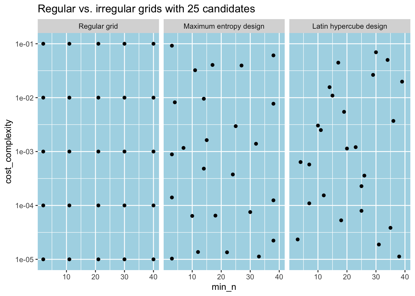

Metric sets

We use performance metrics to assess the predictive performance of our models. tidymodel’s yardstick package provides functions to compute performance metrics for regression and classification problems. Root mean square error (RMSE), mean absolute error (MAE), and R squared are some of the standard regression metrics. yardstick functions for computing performance metrics take in a data argument for data, a truth argument for the actual outcome/response variable, and an estimate argument for the predicted values. Below, we first use augment() to combine the (preprocessed) test data with the fitted/predicted Sale_Price values in a new data frame. augment() uses “.pred” as the column name for the fitted values for consistency across different models. We then pipe the new data to the rmse() function.

augment(tree_fit, ames_test) |>
  rmse(truth = Sale_Price, estimate = .pred)
#> # A tibble: 1 × 3
#>   .metric .estimator .estimate
#>   <chr>   <chr>          <dbl>
#> 1 rmse    standard      0.0947

We can also combine multiple performance metric functions using the metric_set() function in yardstick. metric_set() takes in the bare metric function names and creates a metric set function that computes all those metrics at once. Moreover, the metric set functions follow the same syntax as the individual metric functions. Below, we create a metric set function using the rmse(), rsq, and mae functions and compute the corresponding metrics in one step.

three_metrics = metric_set(rmse, rsq, mae)

augment(tree_fit, ames_test) |>
  three_metrics(truth = Sale_Price, estimate = .pred)
#> # A tibble: 3 × 3
#>   .metric .estimator .estimate
#>   <chr>   <chr>          <dbl>
#> 1 rmse    standard      0.0947
#> 2 rsq     standard      0.692 
#> 3 mae     standard      0.0690

We will see shortly how to use metric sets when tuning. Finally, consider one more helpful function from yardstick: metrics(). This function behaves like the individual metric functions except that what performance metrics it computes depends on the class of the truth argument. For regression problems, it returns RMSE, R², and MAE in a data frame format.

augment(tree_fit, ames_test) |>
  metrics(truth = Sale_Price, estimate = .pred)
#> # A tibble: 3 × 3
#>   .metric .estimator .estimate
#>   <chr>   <chr>          <dbl>
#> 1 rmse    standard      0.0947
#> 2 rsq     standard      0.692 
#> 3 mae     standard      0.0690

Tuning

We are finally ready to tune the model hyperparameters by evaluating the grid. To do so, we can use tune_grid() to fit a simple decision tree model to the 10-fold cross-validation resamples for each combination of parameter values. The grid argument of the function is set to 10 by default and generates a grid using the Latin hypercube design. As we do below, it can also be set to a user-specified grid data frame. We can also specify what performance metrics we want the function to compute by setting its metrics argument to a desired metric set.¹⁵ Below, we only use RMSE. Given that our regular grid contains 25 combinations of parameter values, tune_grid() generates $10 \times 25 = 250$ performance metrics (i.e., RMSE). The .metrics column of tune_results is a list with 10 elements where each element is a data frame that contains RMSE under its .estimate column for each of 25 parameter combinations.

tune_results = 
  tree_wflow |>
  tune_grid(
    resamples = ames_folds,
    grid = grid_reg,
    metrics = metric_set(rmse)
  )
tune_results
#> # Tuning results
#> # 10-fold cross-validation using stratification 
#> # A tibble: 10 × 4
#>    splits             id     .metrics          .notes          
#>    <list>             <chr>  <list>            <list>          
#>  1 <split [2105/237]> Fold01 <tibble [25 × 6]> <tibble [0 × 3]>
#>  2 <split [2106/236]> Fold02 <tibble [25 × 6]> <tibble [0 × 3]>
#>  3 <split [2107/235]> Fold03 <tibble [25 × 6]> <tibble [0 × 3]>
#>  4 <split [2108/234]> Fold04 <tibble [25 × 6]> <tibble [0 × 3]>
#>  5 <split [2108/234]> Fold05 <tibble [25 × 6]> <tibble [0 × 3]>
#>  6 <split [2108/234]> Fold06 <tibble [25 × 6]> <tibble [0 × 3]>
#>  7 <split [2109/233]> Fold07 <tibble [25 × 6]> <tibble [0 × 3]>
#>  8 <split [2109/233]> Fold08 <tibble [25 × 6]> <tibble [0 × 3]>
#>  9 <split [2109/233]> Fold09 <tibble [25 × 6]> <tibble [0 × 3]>
#> 10 <split [2109/233]> Fold10 <tibble [25 × 6]> <tibble [0 × 3]>

autoplot () is a convenient function that can plot the performance metrics against the parameters. We pass in metric = "rmse" to instruct it to plot using RMSE as the performance metric. Since there are only five different min_n values, a different color is used for each to generate a two-dimensional plot. We see that the positive effect of lowering the cost complexity on RMSE diminishes after 0.001. After this point, minimum node sizes 2 and 11 increase RMSE. The minimum node size 21 performs consistently better. The plot suggests we should choose (cost_complexity, min_n) = (0.001, 21) to proceed with our analysis.

autoplot(tune_results, metric = "rmse")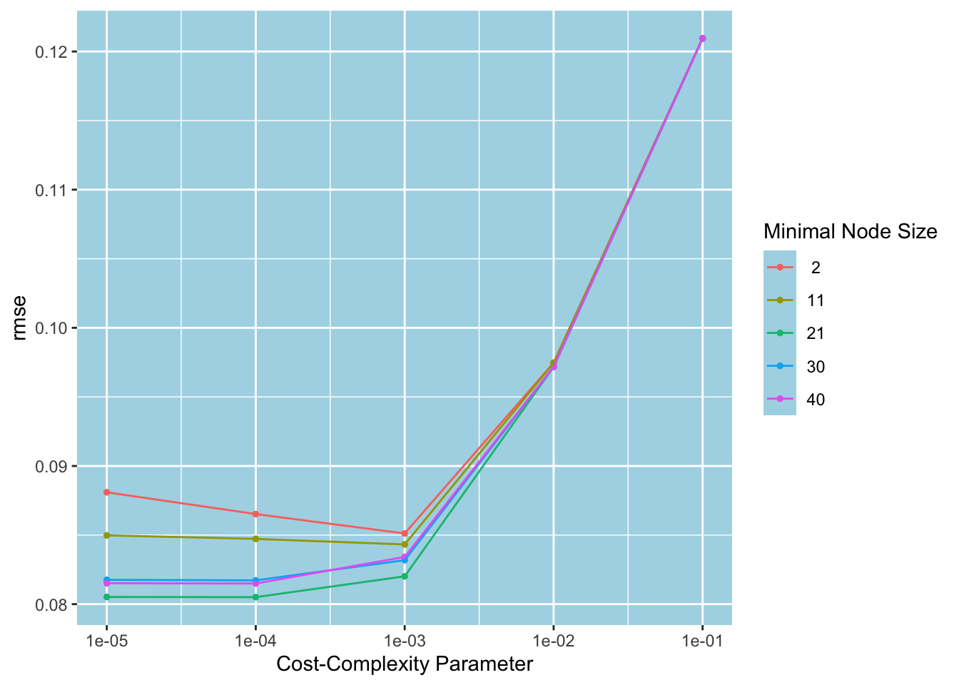

Let’s now tune by evaluating the irregular grid generated by the maximum entropy design. First, we call tune_grid() and save the tuning results.

tune_results_me =
  tree_wflow |>
  tune_grid(
    resamples = ames_folds,
    grid = grid_me,
    metrics = metric_set(rmse)
  )

Below, we plot the tune results. Unlike the regular grid case, we now see a marginal effects plot. The irregular grid designs create too many parameter values to fill in the space, and autoplot() computes the average RMSE for any unique value of a given parameter by averaging RMSE over all values of all other parameters from all assessment sets. As per the cost complexity parameter, the improvement in RMSE stops after 10^-3.5. The case for the minimal node is less clear. It seems that RMSE jumps up suddenly for some points, but it reaches its minimum around 20 observations.

autoplot(tune_results_me, metric = "rmse") +
  labs(title = "Tune results for the maximum entropy design grid")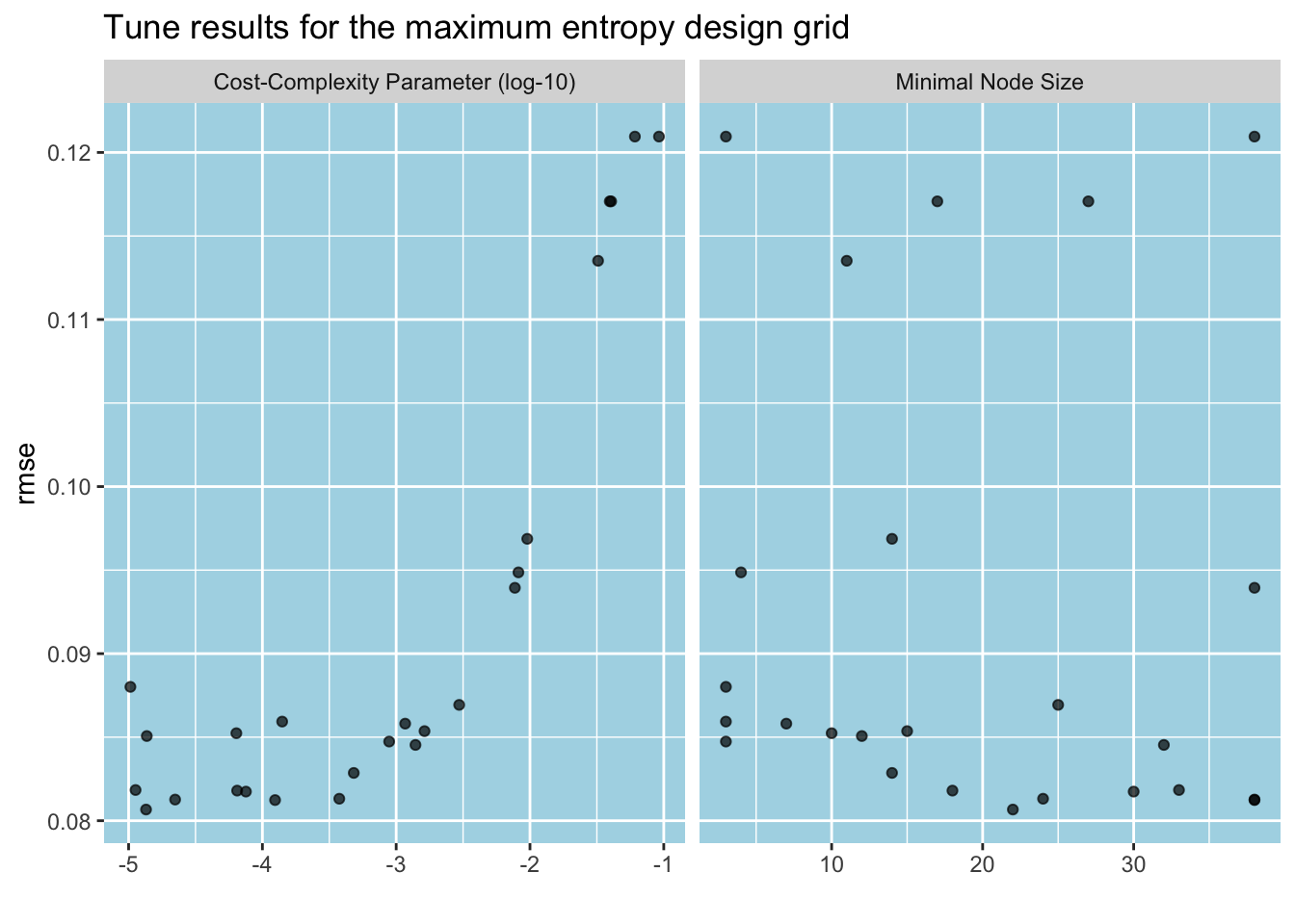

We can view the top five performing candidates using tune’s show_best() function. While the top two are neck and neck, we can pick the first candidate, (cost_complexity, min_n) = (10^-4, 21), to have a simpler tree.

show_best(tune_results, metric = "rmse")
#> # A tibble: 5 × 8
#>   cost_complexity min_n .metric .estimator   mean     n std_err .config         
#>             <dbl> <int> <chr>   <chr>       <dbl> <int>   <dbl> <chr>           
#> 1         0.0001     21 rmse    standard   0.0805    10 0.00304 Preprocessor1_M…
#> 2         0.00001    21 rmse    standard   0.0805    10 0.00304 Preprocessor1_M…
#> 3         0.0001     40 rmse    standard   0.0815    10 0.00280 Preprocessor1_M…
#> 4         0.00001    40 rmse    standard   0.0815    10 0.00279 Preprocessor1_M…
#> 5         0.0001     30 rmse    standard   0.0817    10 0.00303 Preprocessor1_M…

We are all set with tuning. But let me show a different way to use tune_grid() using the Latin hypercube design. The function’s grid argument can be either an integer or a data frame. The function uses the Latin hypercube design as the default choice if its grid argument is set to an integer. So, to use this design, we pass in grid = 25.¹⁶ Since we modified the range for one of our parameters, we must pass in the updated parameter object tree_param to tune_grid(). We set its optional argument param_info to tree_param to do that.

set.seed(345)
tune_results_lh =
  tree_wflow |>
  tune_grid(
    resamples = ames_folds,
    grid = 25,
    param_info = tree_param,
    metrics = metric_set(rmse)
  )

Now that we have selected the best parameter combination, we can use them to finalize the training process. First, we must create a data frame with a column for each parameter and fill it with the best values. We then use finalize_workflow() in the tune package to set the model parameters to their best values. tree_wflow_final can then be fit to the entire Ames data and used to predict with new data.

tree_param_final = tibble(cost_complexity = -4, min_n = 21)

tree_wflow_final = tree_wflow |>
  finalize_workflow(tree_param_final)

Let’s wrap up this section by comparing our tuning with rpart()’s internal tuning. After fitting both our tuned model and rpart’s internally tuned model to the entire training data, we predict with them using the test set and obtain RMSE for each, which will function as the final arbiter.¹⁷ Test RMSE for our tuned model is lower: 0.0760 vs. 0.0947.

Code

rmse1 = tree_wflow_final |>
  fit(ames_train) |>
  augment(ames_test) |>
  rmse(truth = Sale_Price, estimate = .pred) |>
  pull(.estimate)

rmse2 = workflow() |>
  add_formula(Sale_Price ~ .) |>
  add_model(decision_tree(mode = "regression")) |>
  fit(ames_train) |>
  augment(ames_test) |>
  rmse(truth = Sale_Price, estimate = .pred) |>
  pull(.estimate)

sprintf("Test RMSE for self-tuning: %1.4f", rmse1)
#> [1] "Test RMSE for self-tuning: 0.0760"
sprintf("Test RMSE for our tuning:  %1.4f", rmse2)
#> [1] "Test RMSE for our tuning:  0.0947"

Ensembles

Single decision trees are not very good at predictive accuracy, so they are sometimes referred to as weak learners. However, using simple trees as a building block, many trees can be combined to construct an ensemble to serve as a separate predictive model. Unlike their building blocks, ensembles can dramatically improve prediction accuracy. Below, we will consider three different statistical learning methods that rely on the ensemble approach.

Bagged trees

Recall that allowing a single tree to grow deep enough can reduce its bias, but this happens at the expense of high variance. High variance follows from the fact that training the model with different training data leads to significant changes in the split rules, which increases the variance of the predictions.¹⁸. This means that although we obtain a relatively good fit for the training data, the model’s predictions with new data are less reliable. High variance, however, can be reduced by following a well-known statistical principle: averaging.

Bootstrap aggregation, or bagging, is a general method used to reduce the variance of weak learners. In the case of trees, bagging involves growing deep (unpruned) trees from the bootstrapped samples of the training data to obtain (high variance) weak learners. Predictions from each tree are then averaged out to make a final prediction.¹⁹ Individual trees are allowed to grow deep because a) predictions from them will be averaged out to reduce the variance of the final prediction, and b) while they have high variance, they also have low bias due to the bias-variance trade-off. The number of trees that will be bagged is not considered a critical parameter because overfitting is not a concern. In fact, it is turned into an advantage by averaging low-bias high-variance trees. As such, there is no need for hyperparameter tuning in bagging.

Since the bootstrapped samples are used to train trees, the out-of-bag (OOB) observations can be used to compute performance metrics (i.e., error measures) to estimate the test error. Given many trees and possibly large training data sets, using the OOB performance metrics is a computationally cheaper alternative to the k-fold cross-validation approach.

parsnip’s bag_tree() function can specify a bagged tree model. This function uses rpart() as its default computational engine. Since bagging involves growing unpruned trees, the min_n main argument of bag_tree() defaults to 2. Its engine argument cost_complexity defaults to zero. The other engine argument, tree_depth, is set to NULL, which means that it will be later set to 30 by rpart(). bag_tree() needs a parsnip extension package, baguette, to work so we attach it first. Keeping the default choices, we specify a bagged tree model workflow by passing in times = 500 to set_engine() to grow 500 trees for bagging.²⁰ We then fit the model to the training data and obtain test set metrics. Note the improvement in RMSE over a single (tuned) decision tree (0.0566 vs. 0.0760). Lastly, by running bag_fit, you can print the variable importance scores, which we skip.

library(baguette)

bag_spec =
  bag_tree() |>
  set_engine("rpart", method = "anova", times  = 500) |>
  set_mode("regression")

bag_wflow =
  workflow() |>
  add_formula(Sale_Price ~ .) |>
  add_model(bag_spec)

set.seed(123)
bag_fit = fit(bag_wflow, ames_train)

augment(bag_fit, ames_test) |>
  rmse(truth = Sale_Price, estimate = .pred)
#> # A tibble: 1 × 3
#>   .metric .estimator .estimate
#>   <chr>   <chr>          <dbl>
#> 1 rmse    standard      0.0566

Random forests

One major downside of bagging is that individual trees may look alike because splits are likely to be based on the same strong features, particularly early on. This makes trees correlate and reduces the gain from averaging in reducing variance. Random forests are constructed from trees trained on the bootstrapped samples as in bagging. But unlike bagging, only a random sample of $m$ features out of all $p$ features is considered each time a split is attempted. This makes it likely for weaker predictors to be used for splitting. The main advantage of this strategy is that it decorrelates trees and improves upon bagging in reducing variance. Bagging can be considered as a special case of a random forest with $m = p$ .

Hastie et al. (2021) states that $m \approx \sqrt{p}$ is typically chosen for random forests.²¹ In any case, $m$ is a tuning parameter for a random forests (RF) model. The complexity of each tree (for instance, the minimal node size) tends to have a negligible impact on predictive accuracy but is suggested for tuning (Boehmke and Greenwell, 2020). Both in bagging and random forests, picking a relatively large number of trees would be enough to stabilize the error measures.²²

Below, we use parsnip’s rand_forest() function to build an RF model. Its default engine is ranger(), which is a fast implementation of RF. mtry, trees, and min_n are the main arguments of rand_forest() and they all default to NULL. This means that they will be set by ranger() as the (rounded down) square root of the number of features, 500, and 5, respectively.

Next, we tag mtry and min_n by setting them to tune(). We use 1000 trees for the random forest. After creating the model workflow, we extract the parameter set. The question mark under the object column indicates that the parameter range is incomplete. The reason is that the workflow does not know at the moment how many features will be used to fit the model. In our case, this is simply because the dummies are not created yet.

rf_spec =
  rand_forest(mtry = tune(), min_n = tune(), trees = 1000) |>
  set_engine("ranger") |>
  set_mode("regression")

rf_wflow =
  workflow() |>
  add_formula(Sale_Price ~ .) |>
  add_model(rf_spec)

rf_param = rf_wflow |> extract_parameter_set_dials()
rf_param
#> Collection of 2 parameters for tuning
#> 
#>  identifier  type    object
#>        mtry  mtry nparam[?]
#>       min_n min_n nparam[+]
#> 
#> Model parameters needing finalization:
#>    # Randomly Selected Predictors ('mtry')
#> 
#> See `?dials::finalize` or `?dials::update.parameters` for more information.

We can use the finalize() function in dials to determine the final number of features/predictors by passing the training set into it. We now see that tuning will try 74 predictors at most for each split for each tree. However, there will be 73 final features after the dummies are created. It seems that finalize() uses the number of columns in the final data matrix to determine the upper boundary for the parameter range. Given that, we manually set the range for mtry to proceed further.

rf_param |>
  finalize(ames_train) |>
  extract_parameter_dials("mtry")
#> # Randomly Selected Predictors (quantitative)
#> Range: [1, 74]

rf_param = rf_param |>
  update(mtry = mtry(c(1, 73)))

Below, we run tune_grid() to evaluate a regular grid with 25 parameter candidates and plot the tune results. For all minimal node sizes, 19 and 37 random features yield lower RMSE. This suggests that increasing the number of random features beyond what ranger() will use, which is 8, by evaluating floor(sqrt(8)) helps with reducing RMSE. Minimal node size 2 consistently yields lower RMSE.²³

grid_reg = rf_param |> grid_regular(levels=5)

set.seed(313)
tune_results =
  rf_wflow |>
  tune_grid(
    resamples = ames_folds,
    grid = grid_reg,
    metrics = metric_set(rmse)
  )

autoplot(tune_results)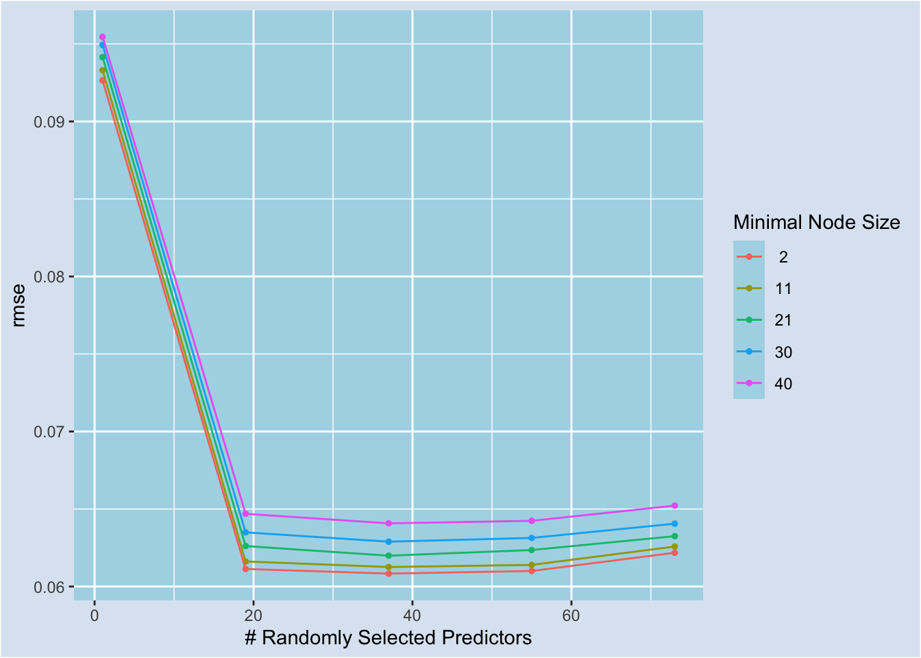

We can view the best five candidates by calling show_best() in the tune package.²⁴ (mtry, min_n) = (37, 2) candidate is the best one.

tune_results |> show_best(metric = "rmse")
#> # A tibble: 5 × 8
#>    mtry min_n .metric .estimator   mean     n std_err .config              
#>   <int> <int> <chr>   <chr>       <dbl> <int>   <dbl> <chr>                
#> 1    37     2 rmse    standard   0.0608    10 0.00331 Preprocessor1_Model03
#> 2    55     2 rmse    standard   0.0610    10 0.00331 Preprocessor1_Model04
#> 3    19     2 rmse    standard   0.0611    10 0.00341 Preprocessor1_Model02
#> 4    37    11 rmse    standard   0.0613    10 0.00335 Preprocessor1_Model08
#> 5    55    11 rmse    standard   0.0614    10 0.00335 Preprocessor1_Model09

Let’s finalize the RF workflow using the best candidate and compute the test set RMSE. We observe a slight improvement over bagging (0.0545 vs. 0.0567).

rf_param_final = tibble(mtry = 37, min_n = 2)

rf_wflow_final = rf_wflow |>
  finalize_workflow(rf_param_final)

set.seed(123)
rf_wflow_final |>
  fit(ames_train) |>
  augment(ames_test) |>
  rmse(truth = Sale_Price, estimate = .pred)
#> # A tibble: 1 × 3
#>   .metric .estimator .estimate
#>   <chr>   <chr>          <dbl>
#> 1 rmse    standard      0.0545

Boosting

Boosting is another general ensemble approach to improve upon the underlying weak learners. Unlike bagging, where trees are grown on the bootstrapped samples independently, trees are grown sequentially in boosting. Each tree uses the residuals generated from the previous tree. Let us consider a numerical example. To start with, we use $0$ to predict the response value for the ith observation so that ${\hat{y_{i}}}^{0} = 0$ . Assume that the actual response value is $y_{i} = 3$ . So the starting residual is $r_{i}^{0} = y_{i} = 3$ . The boosting algorithm uses the starting residual value, 3, as the response value for the ith observation to grow the first tree. Assume that the first grown tree predicts ${\hat{y_{i}}}^{1} = 1$ . The new residual is now $r_{i}^{1} = 3 - 1 = 2$ . The second tree is then fitted to the same feature values by setting the response value to $2$ . Assume that the second tree predicts ${\hat{y_{i}}}^{2} = 0.8$ so that the new residual is $r_{i}^{2} = 2 - 0.8 = 1.2$ . The third tree is again fitted to the same feature values by setting the response value to $1.2$ . Finally, assume that the third tree predicts ${\hat{y_{i}}}^{3} = 0.5$ . This way, each tree tries to fix (i.e., reduce) the prediction error the previous tree failed to reduce by potentially using different features for splitting.

What’s the final prediction for the ith observation? It is computed by adding up the predictions from individual trees. In our example, combining only three trees would yield the predicted response value of (0 plus) $1 + 0.8 + 0.5 = 2.3$ .

Note that, unlike bagging, where trees are grown on the bootstrapped samples, in boosting, trees are grown on the modified version of the original training data, where the modification involves the response values used for each tree. Moreover, simple/shallow trees are preferred in boosting by setting the size of the splits low.²⁵ The reason is that simple trees learn slowly.²⁶ For instance, a more complex first tree would predict $2$ instead of $1$ . The pace of learning can be slowed down further by multiplying the predicted value by a shrinkage parameter (usually less than 0.5), which increases the new residual value to be computed.

There are four main tuning parameters in boosted trees:

the number of trees (or the number of boosting iterations)²⁷,
the shrinkage parameter (the learning rate),
the number of splits in each tree (the tree depth), and
the minimum number of observations in terminal nodes.

The first two are considered boosting hyperparameters, and the latter two can be called tree-specific hyperparameters.²⁸

parsnip’s boost_tree() function can specify a boosted trees model. This function can talk to six underlying packages and uses the xgboost package as its default engine. The package is an R interface for the underlying XGBoost library that implements machine learning algorithms under the gradient boosting framework. The table below shows boost_tree()’s arguments and the corresponding parameters/arguments in xgboost’s xgboost() function side by side, along with a short description and default value from the package documentation.

Mapping from boost_tree() to xgboost()
Arguments/Parameters		Description	Default value
boost_tree()	xgboost()	Description	Default value
learn_rate	eta	control the learning rate: scale the contribution of each tree by a factor of 0 < eta < 1 when it is added to the current approximation	0.3
loss_reduction	gamma	minimum loss reduction required to make a further partition on a leaf node of the tree	0
sample_size	subsample	subsample ratio of the training instance	1
mtry	colsample_bytree	subsample ratio of columns when constructing each tree	1
tree_depth	max_depth	maximum depth of a tree	6
min_n	min_child_weight	minimum sum of instance weight (hessian) needed in a child. In linear regression mode, this simply corresponds to minimum number of instances needed to be in each node	1
trees	nrounds	max number of boosting iterations	15
stop_iter	early_stopping_round	If NULL, the early stopping function is not triggered. If set to an integer k, training with a validation set will stop if the performance doesn't improve for k rounds.	NULL

Below, we tag two tree-specific boosting hyperparameters, tree_depth and min_n, in boost_tree(). We skip tuning the boosting hyperparameters trees and learn_rate for now because the boosting algorithm takes much longer to train as the number of trees gets bigger and the learning rate gets smaller. In the next post, we will also tune these parameters once we learn how to take advantage of parallel processing and different tuning functions to speed up the training process.

xgb_spec = 
  boost_tree(
    trees = 2000, tree_depth = tune(), min_n = tune()
  ) |>
  set_engine("xgboost") |>
  set_mode("regression")

xgb_wflow =
  workflow() |>
  add_formula(Sale_Price ~ .) |>
  add_model(xgb_spec)

xgb_param = xgb_wflow |>
  extract_parameter_set_dials()

set.seed(123)
tune_results =
  xgb_wflow |>
  tune_grid(
    resamples = ames_folds,
    grid = xgb_param |> grid_regular(levels = 3),
    metrics = metric_set(rmse)
  )

With the learning rate set to 0.3 and the number of trees to 2000, the stump (with a tree depth of 1) performs consistently better than deeper trees. However, increasing the minimal node size worsens its performance.

autoplot(tune_results)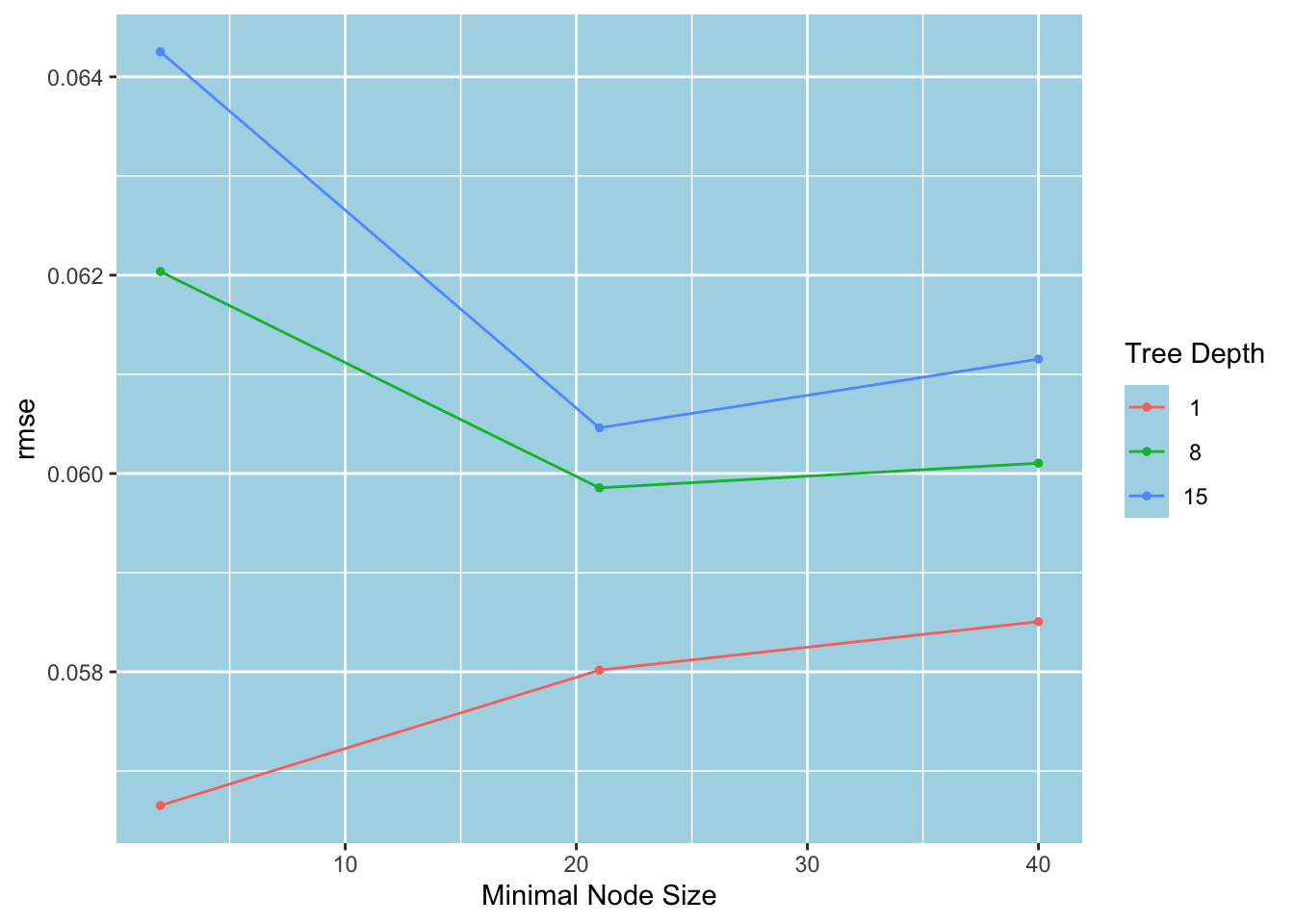

Below, we see that (min_n, tree_depth) = (2, 1) is the best candidate.

show_best(tune_results, metric = "rmse")
#> # A tibble: 5 × 8
#>   min_n tree_depth .metric .estimator   mean     n std_err .config             
#>   <int>      <int> <chr>   <chr>       <dbl> <int>   <dbl> <chr>               
#> 1     2          1 rmse    standard   0.0567    10 0.00359 Preprocessor1_Model1
#> 2    21          1 rmse    standard   0.0580    10 0.00339 Preprocessor1_Model2
#> 3    40          1 rmse    standard   0.0585    10 0.00309 Preprocessor1_Model3
#> 4    21          8 rmse    standard   0.0599    10 0.00344 Preprocessor1_Model5
#> 5    40          8 rmse    standard   0.0601    10 0.00300 Preprocessor1_Model6

We now finalize the boosted trees workflow using the best candidate and compute the test RMSE.

xgb_param_final = tibble(min_n = 2, tree_depth = 1)

xgb_wflow |>
  finalize_workflow(xgb_param_final) |>
  fit(ames_train) |>
  augment(ames_test) |>
  rmse(truth = Sale_Price, estimate = .pred)
#> # A tibble: 1 × 3
#>   .metric .estimator .estimate
#>   <chr>   <chr>          <dbl>
#> 1 rmse    standard      0.0476

We tuned only two parameters, and the boosted trees model still improved upon the RF model by almost 13% (0.0476 vs. 0.0545).

Summary

In this post, we have focused on tree-based models and how to tune them. A decision tree can be used as a building block to create ensembles that significantly improve predictive accuracy. Bagged trees, random forests, and boosted trees are ensembles, each leveraging a different strategy for using single trees. With tidymodels, we can easily tune hyperparameters of single trees, random forests, and boosted trees. In the next post, we will learn about parallel processing and different tuning strategies that allow us to conduct tuning faster.

Footnotes

This is due to limited space. We will see the full names below.↩︎
The Gini impurity index or entropy are used for classification problems since SSE cannot be used as a criterion for making the splits in this case. To see how these measures are defined, see Hastie et al. (2021).↩︎
This function is provided by rpart package. Below, we still pass in “rpart” to set_engine() for clarity.↩︎
For instance, rpart() sets (maximum) tree depth to 30, minimum node size to 20, and cost complexity to 0.01.↩︎
In this case, the function grabs the scores from the fit object created by the underlying engine rpart(). You can run tree_fit$variable.importance to view the raw VI scores. You can also use the vi() function in vip to obtain VI scores in a data frame format. Run vip::vi(tree_fit) to do so.↩︎
tune_bayes() is an alternative for Bayesian optimization of model parameters. tune_race_anova() in the finetune package also tunes. We will learn about this function in the next post.↩︎
If you want an unpruned tree, you can set cost_complexity to zero, in which case there is no need for tuning.↩︎
This saves around 6 seconds per 10-fold cross-validation tune run on my machine.↩︎
Using a transformer function might seem confusing. However, it saves us from typing 0.0000000001 in this instance.↩︎
These functions are in the hardhat package that is also included in tidymodels meta-package.↩︎
Run tree_param$object[[1]] to see this.↩︎
We will see shortly how this updated parameter object could be used.↩︎
Whether the range is on the transformed scale or not affects the values. In our case, the range for the cost complexity parameter is on the transformed scale, and the step size to create those five values is computed as $(- 1 - (- 5)) / (5 - 1) = 1$ . That’s why, for instance, the second value is $10^{- 5 + 1} = 0.0001$ .↩︎
grid_random(), on the other hand, picks parameter values from a uniform distribution whose range is the same as the parameter range. For up to mid-size grids, it may return overlapping values.↩︎
This argument is optional; when not specified, the function computes the standard metrics.↩︎
Due to randomness involved in irregular grid designs, we use the same seed number that we used above.↩︎
rpart() returns a fit object whose cptable contains the cross-validation error against the cost complexity parameter. Run extract_fit_engine(tree_fit)$cptable to see that the lowest CV error occurs when cp = 0.01, which was used to generate the tree chart we plotted at the top.↩︎
This is intrinsic to the model in that its structure determines where it stands on the bias-variance trade-off spectrum.↩︎
In classification problems, a majority vote rule is used to determine the predicted class.↩︎
As far as I can see, there is no argument in rpart() that corresponds to times. It seems that bag_tree() uses times to run rpart() that many times.↩︎
Boehmke and Greenwell (2020) states that $m = floor (p / 3)$ is the preferred starting point for regression problems.↩︎
Boehmke and Greenwell (2020) suggests $p \times 10$ trees as a good rule of thumb.↩︎
One can create a denser grid to find better candidates as well. It is very likely that this will not lead to a dramatic improvement in RMSE. Plus, due to the large number of trees, tuning will take significantly longer.↩︎
select_best() will return the row that contains the best candidate.↩︎
It can be as low as 1. One split implies a stump.↩︎
Note here a main difference between bagging and boosting strategies. While bagging tries to turn high variance into an advantage by averaging, boosting tries to turn high bias into an advantage by sequentially improving upon the bias.↩︎
Unlike bagging and random forests, where predictions are averaged out, using too many trees to boost can lead to overfitting.↩︎
See Boehmke and Greenwell (2020).↩︎