Machine Learning with tidymodels – Part 1

Fundamental steps

Published

Jan 15, 2025

tidymodels is a meta-package for machine learning and statistical analysis in R. It offers tools to greatly simplify the model training process. Moreover, it shares the same design principles as the tidyverse package, including clear function names, the ability to work with the pipe operator, and returning results as tidy data. In several blog posts, including this one, I will show how to use tidymodels to train the leading machine learning models in R.¹ This first post of the series will focus on random data splitting, preprocessing features, model specification, and model training.² We will determine what features fetch higher or lower home sale prices using a residential data set. Does, for instance, the lot shape of the house matter? Let’s find out.

Go ahead and run install.packages("tidymodels") in your R console to download and install the tidymodels package on your machine. To attach it, run

library(tidymodels)
#> ── Attaching packages ────────────────────────────────────── tidymodels 1.2.0 ──
#> ✔ broom        1.0.6     ✔ recipes      1.1.0
#> ✔ dials        1.3.0     ✔ rsample      1.2.1
#> ✔ dplyr        1.1.4     ✔ tibble       3.2.1
#> ✔ ggplot2      3.5.1     ✔ tidyr        1.3.1
#> ✔ infer        1.0.7     ✔ tune         1.2.1
#> ✔ modeldata    1.4.0     ✔ workflows    1.1.4
#> ✔ parsnip      1.2.1     ✔ workflowsets 1.1.0
#> ✔ purrr        1.0.2     ✔ yardstick    1.3.1
#> ── Conflicts ───────────────────────────────────────── tidymodels_conflicts() ──
#> ✖ purrr::discard() masks scales::discard()
#> ✖ dplyr::filter()  masks stats::filter()
#> ✖ dplyr::lag()     masks stats::lag()
#> ✖ recipes::step()  masks stats::step()
#> • Dig deeper into tidy modeling with R at https://www.tmwr.org

The printed message shows the attached packages and function conflicts. tiydmodels provides a function that prioritizes its functions over the conflicted ones. To do so, run

tidymodels_prefer()

The nine packages out of the eighteen packages included in the meta-package are distinct to tidymodels: rsample, parsnip, recipes, workflows, workflowsets, tune, yardstick, dials, infer and modeldata. The table below shows the main functionality of each package. The remaining nine packages are the familiar tidyverse packages that make it easier to work with tidymodels.

Core Tidymodels Packages and Their Main Functionality
Package	Functionality
rsample	random data splitting and resampling
parsnip	model specification functions and model training
recipes	model equation/formula and preprocessing functions
workflows	workflow structure to combine recipes with model specifications
workflowsets	workflow sets for training multiple models together
yardstick	regression and classification metrics
tune	hyperparameters tuning
dials	grids and parameter objects for tuning
infer	statistical inference
modeldata	example data sets

Splitting and resampling data with rsample

In this part, we will see how we can use the functions offered by the rsample package to split available data and generate resamples to compute performance metrics or tune hyperparameters.

Loading data and initial inspection

We will work on the Ames data set included in tidymodels’ modeldata package. This data set contains information about 2930 individual residential properties sold in Ames, Iowa, from 2006 to 2010.³ All non-numeric columns in it are already formatted as factor variables. Interestingly, it includes a variable called Sale_Price (the last sale price of properties) along with other variables that capture their different features such as Overall_Cond, Neighborhood, Year_Built, Gr_Liv_Area (above-ground living area), and so on. We can use this data set to predict the sale price of a house based on its features. In this setting, sale price is an outcome or response variable, and the other variables used to predict it are predictors (or features).

Let’s load the data and check its dimensions.

data(ames)
dim(ames)
#> [1] 2930   74

What does the distribution of sale price look like? Let’s plot a histogram to get an idea. The following plot suggests that the distribution of the sale price is right-skewed.

ggplot(ames, aes(Sale_Price)) +
  geom_histogram(bins = 100, color = "white")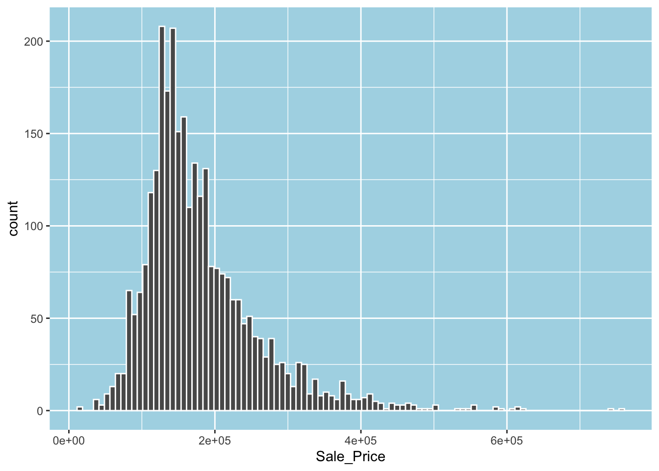

Applying a log transformation to Sale_Price will attenuate the right skewness and drive it towards a normal distribution.⁴ Let’s log transform Sale_Price and replace the original with the log-transformed one.

ames = mutate(ames, Sale_Price = log10(Sale_Price))

As expected, the log-transformed variable looks more normal. Note that there are still outliers, but there are fewer now.

ggplot(ames, aes(Sale_Price)) +
  geom_histogram(bins = 100, color = "white") +
  labs(x = "Sale Price (log)")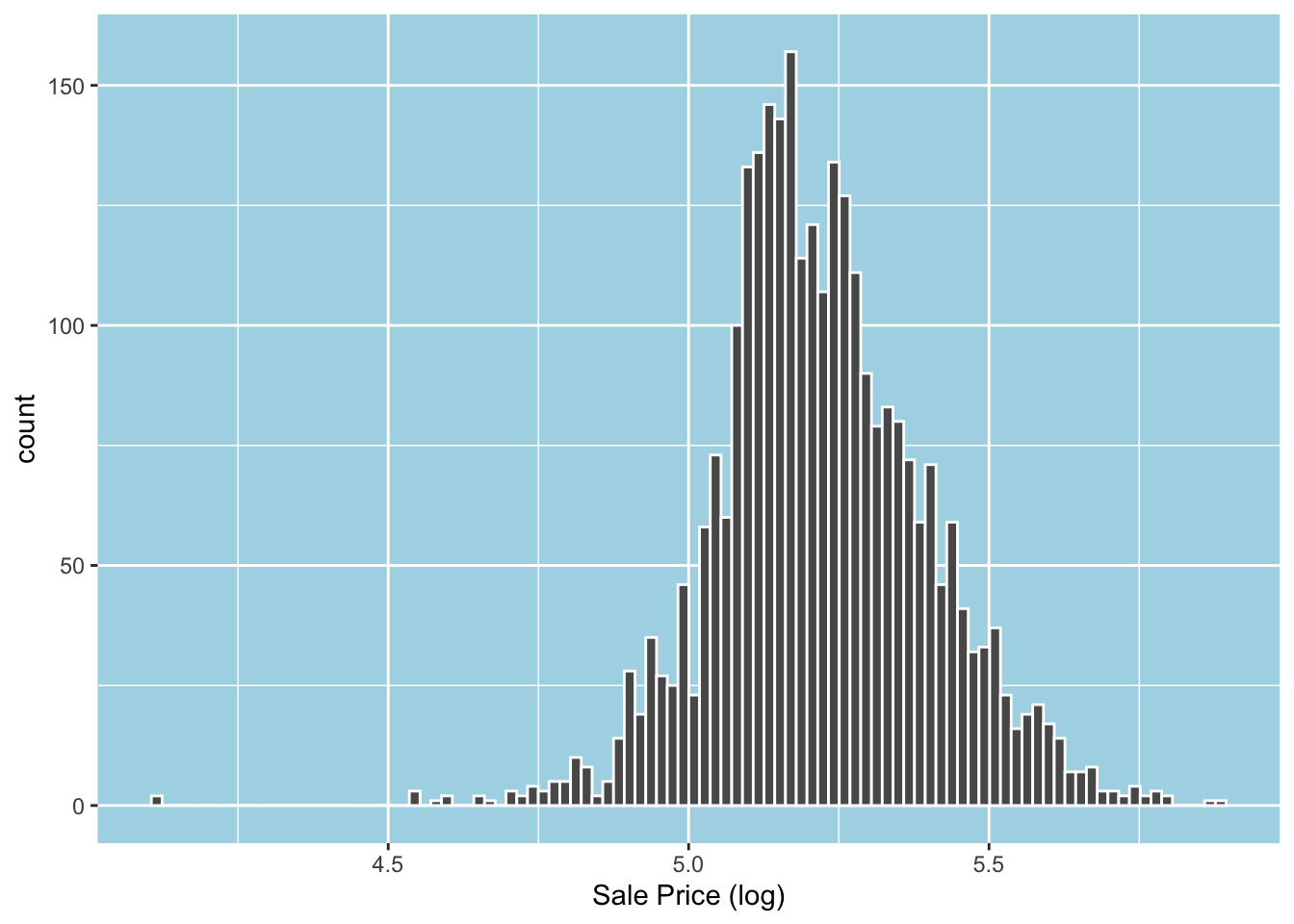

Before creating training and test sets, we should check if our data contains any missing values, which we should deal with if possible. As we see below, there is no missing value in our data.⁵

sum(is.na(ames))
#> [1] 0

Splitting data

Basic splitting

A standard initial procedure in any statistical learning exercise is to place (or spend) the majority of available data (or the data budget) in a training set and the remaining data in a test set. A data science practitioner uses the training set to train and optimize models. The test set is only used to assess the model’s performance once the model training process is complete. The rsample package provides functions that split the overall data into training and test tests. Below, we see how to use the initial_split() function to perform basic splitting.

set.seed(2025)
ames_split = initial_split(ames, prop = 0.8, strata = Sale_Price)
ames_split 
#> <Training/Testing/Total>
#> <2342/588/2930>

Random data splitting involves randomly picking some row numbers from a given data. ames_split is an rsplit list that contains a vector named in_id that has the randomly picked row numbers as its elements.⁶ The observations in the selected rows will be included in the training set. Running ames_split prints the number of observations slated for the training and test sets. The training set includes almost 80% of the total observations, as we wanted by setting the prop argument to 0.8.

While randomly splitting data into training and test sets is a good idea, there is no guarantee that the distribution of the outcome/response variable will be the same across the sets. To ensure this, the initial_split() function accepts a strata argument to use stratification in random sampling. For numeric variables like our Sale_Price, data are binned into quartiles, and then splitting is applied to each quartile.⁷

To generate the training and test sets, we pass in the rsplit object to training() and testing() functions, provided again rsample:

ames_train = training(ames_split)
ames_test = testing(ames_split)

Resampling

A fundamental procedure for empirical model evaluation involves partitioning the training data multiple times to allocate some data for training and different data for evaluation each time. This is known as resampling. Kuhn and Silge (2023) call the set that includes most of the training data analysis set and the set that consists of the remaining training data assessment set. The analysis set is used to train/fit a model, and the assessment set is used to obtain performance metrics for the trained model. The model that generates the best performance metric(s) against the assessment sets is picked for the final evaluation of the model against the test set that was created in the previous step.

Why resampling? As we train our models by either adding additional variables or adjusting/tuning the model hyperparameters (e.g., the number of hidden units in a neural net, the number of trees in a decision tree, the number of nearest neighbors, etc.), we use the assessment set to measure the model performance. Most statistical models estimate their parameters by optimizing a specific metric based on prediction errors to obtain the best fit. Moreover, we can use sophisticated model specifications (e.g., interaction and quadratic terms in a linear model) or specific model hyperparameter values to improve the fit further. However, these actions do not guarantee success in prediction with new data, which is the whole point of statistical learning in many settings. Oftentimes, the model learns too much during the training process, and it underperforms when it faces new data. This is known as overfitting. Using the assessment sets to obtain performance metrics, we can assess the predictive success of the model without referring to the performance metrics associated with the analysis set. In other words, we empirically validate our model in a non-self-referential way. This is where the main benefit of resampling lies.

Cross-validation

A standard resampling method is called cross-validation. It involves randomly splitting training data into $v$ sets (aka folds) where each observation belongs to only one set so that the sets are mutually exclusive. One fold is reserved as the assessment set (called holdout). The remaining $v - 1$ folds are combined to form the analysis set. Since a different fold is held out as the assessment set and the remaining $v - 1$ folds are combined to form the analysis set, this resampling process yields $v$ analysis and $v$ assessment sets. This way, rather than fitting the model to a single training set and measuring its performance against the corresponding single test set, training and testing are conducted $v$ times. Moreover, this routine can be repeated multiple times (i.e., repeated cross-validation).

rsample’s vfold_cv() function performs this task.⁸ It takes a $v$ argument for the number of splits and a repeats argument for the number of times splitting is done.⁹ The function returns a tibble object where each row contains an rsplit object storing the partitioning information and an id string to represent the fold and/or repeat.

set.seed(342)
ames_folds = 
  vfold_cv(
    ames_train,
    v = 10, 
    repeats = 1, 
    strata = Sale_Price
  )

ames_folds works just like ames_split in that it contains only the partitioning information, which is contained as row numbers in the in_id vector of the splits list.¹⁰

The rsample package offers analysis() and assessment() functions to extract the data allocated for the corresponding sets. Both functions need an rsplit object containing the split information. For instance, you can run analysis(ames_folds$splits[[10]]) to extract the analysis set data for the tenth split.

Validation sets

Another resampling method involves partitioning the overall data into three sets: a training, a validation, and a test set. rsample’s initial_validation_split() function splits the data in three. The prop argument expects a two-element vector to represent the proportions of data that will go to the training and validation sets, respectively. For instance, prop = c(0.6, 0.2) instructs the function to put approximately 60% of data to training, 20% to validation, and 20% to test set.

set.seed(184)
ames_val_split = 
  initial_validation_split(
    ames_train, 
    prop = c(0.6, 0.2),
    strata = Sale_Price
    )
ames_train = training(ames_val_split)
ames_val = validation(ames_val_split)
ames_test = testing(ames_val_split)

Bootstrapping

Unlike the previous resampling methods, bootstrapping randomly selects observations with replacement from the training data. Moreover, in bootstrapping, the analysis set contains the same number of observations as the training set. Random selection with replacement means that the same observations can be placed in the analysis set more than once. The observations that are not selected at all for inclusion in the analysis set form the assessment set (which is commonly referred to as the “out-of-bag” (OOB) sample). rsample’s bootstraps() function generates bootstrap resamples. The function accepts a times argument for the number of bootstrap samples and a strata argument for the stratification variable within which the random sampling is conducted.

set.seed(547)
ames_boots = bootstraps(ames_train, times = 10, strata = Sale_Price)

Note that each split has the same number of observations (2342) as the training set, but the size of the analysis sets differs across the resamples.

We have considered the main methods for resampling.¹¹ It is now time to move on to the next step.

Preprocessing with recipes

Now that we have decided how to spend our data, it is time to work on the model. A fundamental first step is to state the outcome variable and predictors and preprocess them to potentially increase the efficiency of machine learning models and to meet the computational expectations of the corresponding algorithms.¹²

Model formula/equation

Let’s assume that the sale price of a house depends on the above-ground living area (in square feet), its neighborhood, and overall condition. The recipe() function in the recipes package has a regular formula argument for stating the outcome variable and predictors, and a data argument. recipe() uses the data to check if the variables provided in the formula exist in the data and to determine their data type. The function returns a recipe object, which is a list.

ames_rec = 
  recipe(
    Sale_Price ~ Gr_Liv_Area + Neighborhood + Overall_Cond, 
    data = ames_train
  )
ames_rec
#> 
#> ── Recipe ──────────────────────────────────────────────────────────────────────
#> 
#> ── Inputs
#> Number of variables by role
#> outcome:   1
#> predictor: 3

ames_rec list object stores all variable names stated in the formula in the variable column of its var_info tibble. The column type stores the data type, and the column role stores the role of the variable (i.e., whether they are “predictor” or “outcome”).¹³

What if we want to have a model where we use all predictors? We can put a . on the right-hand side of ~ to use all predictors in the model formula as follows:

ames_rec = recipe(Sale_Price ~ ., data = ames_train)
ames_rec
#> 
#> ── Recipe ──────────────────────────────────────────────────────────────────────
#> 
#> ── Inputs
#> Number of variables by role
#> outcome:    1
#> predictor: 73

Feature engineering

There are several essential checks we should do before proceeding to training a model. For instance, we should ensure that our predictors are informative enough; hence, it would be helpful to include them in the model. A basic condition for any predictor to be helpful is to have some variance across observations. We may want to check whether predictors have zero variance (i.e. if they contain one unique value) or near zero variance. The nearZeroVar() function in the caret package checks if predictors have zero or near zero variance.¹⁴ We see below that 20 features in our data set have near zero variance (and no feature has zero variance).

caret::nearZeroVar(ames_train, saveMetrics = TRUE) |>
  rownames_to_column() |>
  filter(nzv == TRUE | zeroVar == TRUE)
#>               rowname  freqRatio percentUnique zeroVar  nzv
#> 1              Street  259.22222     0.0853971   FALSE TRUE
#> 2               Alley   22.75000     0.1280956   FALSE TRUE
#> 3        Land_Contour   21.24242     0.1707942   FALSE TRUE
#> 4           Utilities 2341.00000     0.0853971   FALSE TRUE
#> 5          Land_Slope   21.18095     0.1280956   FALSE TRUE
#> 6         Condition_2  231.70000     0.3415884   FALSE TRUE
#> 7           Roof_Matl  115.35000     0.2988898   FALSE TRUE
#> 8           Bsmt_Cond   23.88636     0.2561913   FALSE TRUE
#> 9      BsmtFin_Type_2   23.70238     0.2988898   FALSE TRUE
#> 10            Heating  100.21739     0.2561913   FALSE TRUE
#> 11      Kitchen_AbvGr   21.70874     0.1280956   FALSE TRUE
#> 12         Functional   36.86441     0.3415884   FALSE TRUE
#> 13      Open_Porch_SF   22.45652     9.8206661   FALSE TRUE
#> 14     Enclosed_Porch  124.18750     6.9598634   FALSE TRUE
#> 15 Three_season_porch  772.00000     0.9820666   FALSE TRUE
#> 16       Screen_Porch  194.00000     4.6114432   FALSE TRUE
#> 17          Pool_Area 2330.00000     0.5550811   FALSE TRUE
#> 18            Pool_QC  582.50000     0.2134927   FALSE TRUE
#> 19       Misc_Feature   30.09333     0.2134927   FALSE TRUE
#> 20           Misc_Val  161.42857     1.3663535   FALSE TRUE

Given the previous finding, we should remove the near-zero variance features from the model. This is where recipes’ step_*() functions come in handy. The relevant function here is step_nzv(). The step functions must be told which variables (outcome or features) will be subject to the corresponding feature engineering step implied by the function. Below, we use the all_predictors() function to select all predictors to be checked for near-zero variance.¹⁵

ames_rec =
  recipe(Sale_Price ~ ., data = ames_train) |>
  step_nzv(all_predictors()) 
ames_rec
#> 
#> ── Recipe ──────────────────────────────────────────────────────────────────────
#> 
#> ── Inputs
#> Number of variables by role
#> outcome:    1
#> predictor: 73
#> 
#> ── Operations
#> • Sparse, unbalanced variable filter on: all_predictors()

The message returned after running ames_rec now includes operations information to tell us that when the model is actually trained/fitted, all features that have near zero variance will be removed from the model equation.¹⁶

Another important thing to check concerns numeric variables. Some models, such as generalized linear models (GLMs), assume a normal distribution of predictors (and the outcome). In such cases, one can rely on the Box-Cox or Yeo-Johnson transformation to drive data towards normality. The former requires input variables to be strictly positive.¹⁷ The recipes package has step_BoxCox() and step_YeoJohnson() functions for the Box-Cox and Yeo-Johnson transformation, respectively.

As we have seen before, applying a log transformation to a variable will also reduce the right-skewness and move it towards normality. In fact, Gr_Liv_Area, just like Sale_Price, is right-skewed, and the log transformation will remove much of its skewness:

p1 = ggplot(ames_train, aes(Gr_Liv_Area)) + 
  geom_histogram(bins = 75, color = "white")

p2 = p1 + scale_x_log10() 

gridExtra::grid.arrange(p1, p2, ncol = 2)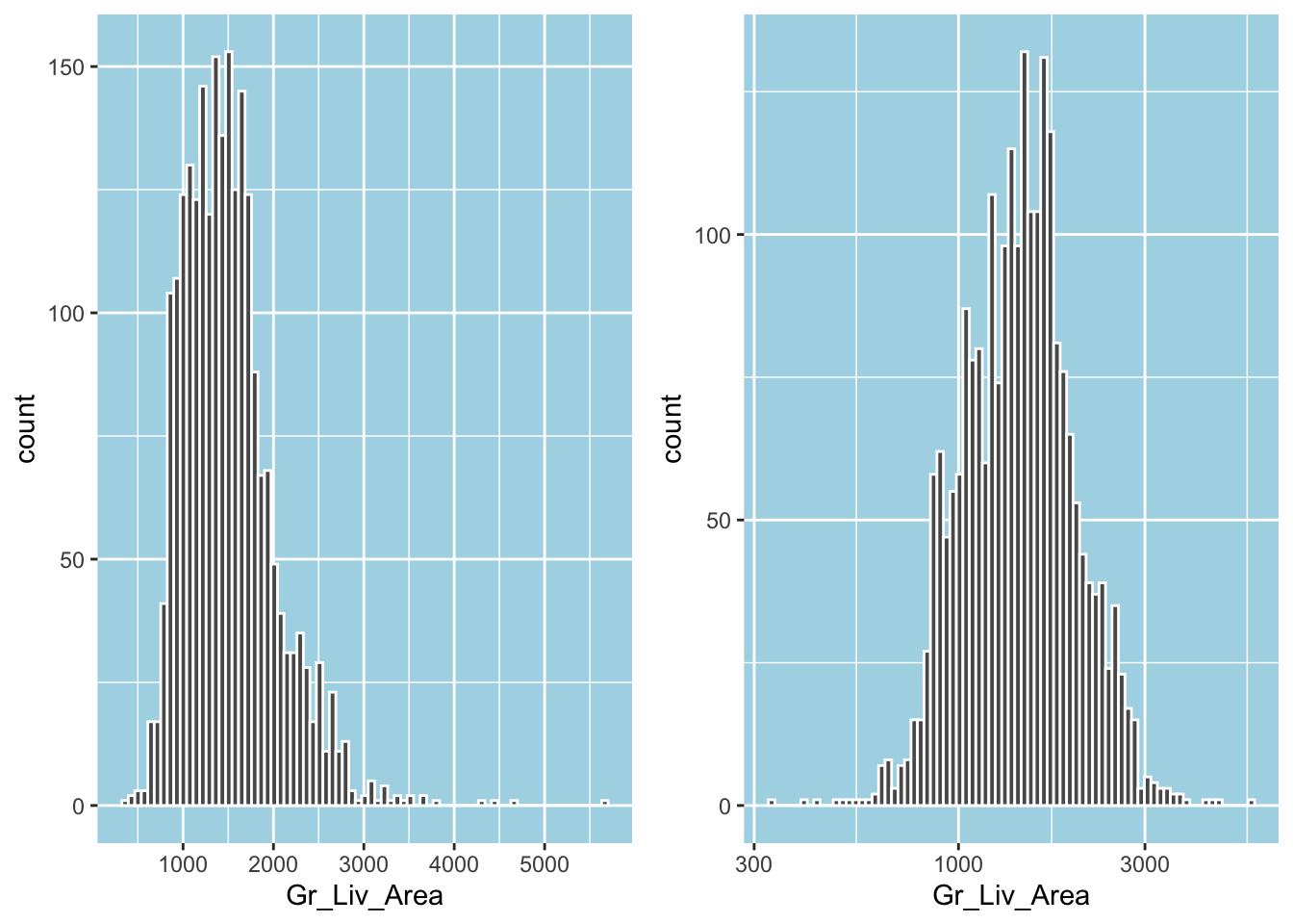

We can use the step_log() function to log-transform a predictor. Below, we apply it to Gr_Liv_Area by setting the logarithmic base to 10.

ames_rec = 
  recipe(Sale_Price ~ ., data = ames_train) |>
  step_log(Gr_Liv_Area, base = 10)
ames_rec
#> 
#> ── Recipe ──────────────────────────────────────────────────────────────────────
#> 
#> ── Inputs
#> Number of variables by role
#> outcome:    1
#> predictor: 73
#> 
#> ── Operations
#> • Log transformation on: Gr_Liv_Area

For some other models to be run efficiently, such as neural nets, k-nearest neighbors, and support vector machines, predictors must be centered and scaled (i.e., standardized or normalized) to have zero mean and unit variance. To standardize, we can use the step_normalize() function by passing into it all_numeric_predictors() to select all numeric features as follows:

ames_rec =
  recipe(Sale_Price ~ ., data = ames_train) |>
  step_normalize(all_numeric_predictors())
ames_rec
#> 
#> ── Recipe ──────────────────────────────────────────────────────────────────────
#> 
#> ── Inputs
#> Number of variables by role
#> outcome:    1
#> predictor: 73
#> 
#> ── Operations
#> • Centering and scaling for: all_numeric_predictors()

So far, we have considered some preprocessing operations available mainly for numeric variables. What about categorical variables? What key feature engineering steps would make sense to apply to them?

Many machine learning algorithms require categorical variables to be converted into numeric counterparts, and a typical conversion involves creating dummy variables. However, sometimes categorical variables would have some levels with a very low frequency in the sample. In such cases, it would make sense to collapse these levels into an arbitrary level so that the number of dummies created will be limited. In our data set, Neighborhood has a few levels with a very low frequency.

ames_train |> 
  count(Neighborhood) |>
  mutate(freq = 100 * (n / nrow(ames_train))) |>
  arrange(freq)
#> # A tibble: 28 × 3
#>    Neighborhood            n   freq
#>    <fct>               <int>  <dbl>
#>  1 Green_Hills             1 0.0427
#>  2 Landmark                1 0.0427
#>  3 Blueste                 6 0.256 
#>  4 Greens                  8 0.342 
#>  5 Veenker                18 0.769 
#>  6 Northpark_Villa        19 0.811 
#>  7 Bloomington_Heights    21 0.897 
#>  8 Briardale              28 1.20  
#>  9 Meadow_Village         31 1.32  
#> 10 Clear_Creek            33 1.41  
#> # ℹ 18 more rows

Given these low frequencies, we can preprocess Neighborhood with step_other() by passing in a frequency threshold value, say 1% as 0.01, to lump the neighborhoods with frequencies lower than the threshold value to the “other” category.¹⁸ Seven neighborhoods will be lumped into the “other” category with the following recipe step.

ames_rec = 
  recipe(Sale_Price ~ ., data = ames_train) |>
  step_other(Neighborhood, threshold = 0.01)
ames_rec
#> 
#> ── Recipe ──────────────────────────────────────────────────────────────────────
#> 
#> ── Inputs
#> Number of variables by role
#> outcome:    1
#> predictor: 73
#> 
#> ── Operations
#> • Collapsing factor levels for: Neighborhood

A further inspection of the data indicates that some other variables, such as Overall_Cond, Electrical, and Garage Finish, also contain levels with less than 1% frequency. However, unlike Neighborhood, the number of such levels within them is minimal, suggesting that resorting to lumping would not yield much.

How do we create numeric variables to represent the information in categorical variables so that machine learning algorithms can process them? The most common method is to encode the information in a categorical variable by creating dummy variables that take on only two values, 0 or 1. There are two options here: one-hot encoding and dummy encoding. The one-hot encoding creates the same number of dummy variables as the number of levels in a categorical variable. The dummy encoding, which is quite common in GLMs settings, creates one less dummy variable than the number of levels in a categorical variable. Both can be easily achieved with the step_dummy() function in recipes. We pass in all_nominal_predictors() function to select all categorical predictors in the data to encode them.

# one-hot encoding
ames_rec = 
  recipe(Sale_Price ~ ., data = ames_train) |>
  step_dummy(all_nominal_predictors(), one_hot = TRUE)

# dummy encoding
ames_rec = 
  recipe(Sale_Price ~ ., data = ames_train) |>
  step_dummy(all_nominal_predictors())

As I pointed out above, the step functions perform preprocessing only when the model is trained/fitted (or a recipe is prepared or baked, which we will get to shortly). Until then, the steps are just steps to indicate how we want to preprocess the data.

The step_dummy() function will use the following naming convention to create dummy variables: the original variable name and factor levels will be concatenated via an _. For instance, the dummies that will be made out of Overall_Cond, which contains such levels as “Very_Poor”, “Poor”, etc., will be named “Overall_Cond_Very_Poor”, “Overall_Cond_Poor” and so on.

It is important to note that when categorical variables are stored as factor variables in a given data set, they retain all factor levels even if the data is partitioned through random splitting for training/testing by R. For instance, Overall_Cond has a level named “Very_Excellent” but there is no observation with this value in either the training or test set. Moreover, each of the variables, including Exterior_1st, Exterior_2nd, and Mas_Vnr_Type, has one particular level for which there are no corresponding observations in the training set either because there are simply no such observations in the overall data or because random splitting happened to place all observations with that value in the test set. In all these cases, when the step_dummy() function creates dummies, it will create dummies for those missing factor levels anyway since it uses all factor levels. This is useful because it allows us to encode these levels, which the model can come across either in the test set or when it is deployed for prediction, and it will still be able to predict.¹⁹

The recipe package offers numerous step*() functions, and we cannot review them here. For the complete list, see the package function reference page.

Putting it all together

Once we decide on the initial feature engineering steps, we can combine step_*() functions using the pipe operator to create a fairly sophisticated recipe or preprocessor. Below, we combine six preprocessing steps. step_*() functions work like dyplr’s select() function. For instance, we can use a - to exclude variables from being preprocessed. Since we log-transform Gr_Liv_Area in a previous step, we exclude it from the Yeo-Johnson transformation step for illustration.²⁰

ames_rec = 
  recipe(Sale_Price ~ ., data = ames_train) |>
  step_nzv(all_predictors()) |>
  step_log(Gr_Liv_Area, base = 10) |>
  step_YeoJohnson(all_numeric_predictors(), -Gr_Liv_Area) |>
  step_normalize(all_numeric_predictors()) |>
  step_other(Neighborhood, threshold = 0.01) |>
  step_dummy(all_nominal_predictors())

Before we wrap up preprocessing, let’s see what the prep() and bake() functions do. In some feature engineering steps, certain quantities and statistics (or computations) must be generated, such as the mean and standard deviation in a standardization step. Such computations will then be used to predict using new data or obtain performance metrics against the assessment or test set. The prep() function generates such computations and uses them to transform the original training/analysis data provided to it. In turn, the bake() function uses these computations to transform the new data. The bake() function also accepts the training/analysis data to transform it. The transformed data is the final data the machine learning algorithms use to fit/train a model.

ames_prep = ames_rec |>
  prep(training = ames_train)

ames_prep
#> 
#> ── Recipe ──────────────────────────────────────────────────────────────────────
#> 
#> ── Inputs
#> Number of variables by role
#> outcome:    1
#> predictor: 73
#> 
#> ── Training information
#> Training data contained 2342 data points and no incomplete rows.
#> 
#> ── Operations
#> • Sparse, unbalanced variable filter removed: Street and Alley, ... | Trained
#> • Log transformation on: Gr_Liv_Area | Trained
#> • Yeo-Johnson transformation on: Lot_Frontage and Lot_Area, ... | Trained
#> • Centering and scaling for: Lot_Frontage and Lot_Area, ... | Trained
#> • Collapsing factor levels for: Neighborhood | Trained
#> • Dummy variables from: MS_SubClass, MS_Zoning, Lot_Shape, ... | Trained

Note that the printed message’s operations section now includes “Trained”. We can say that the prep() function trains the recipe by implementing the preprocessing steps.

A comparison of ames_rec and ames_prep is illustrative. We see that ames_prep is still a recipe list with the same structure as ames_rec.²¹ The var_info tibble in both of them is the same. Unlike ames_rec, ames_prep’s term_info tibble now contains the name of the variables created after preprocessing steps are implemented, and it has 207 rows, indicating that model training will involve 207 variables. Moreover, unlike ames_rec’s template tibble that contains the original training data, ames_prep’s template contains the final preprocessed training data with 207 variables. The exact final data can be generated using the bake() function by providing it with the training/analysis data.²²

ames_baked = ames_prep |> bake(new_data = ames_train)
ames_baked
#> # A tibble: 2,342 × 207
#>    Lot_Frontage Lot_Area Year_Built Year_Remod_Add Mas_Vnr_Area BsmtFin_SF_1
#>           <dbl>    <dbl>      <dbl>          <dbl>        <dbl>        <dbl>
#>  1     0.667       0.525    -0.351         -1.12         -0.794        0.836
#>  2     0.406      -0.135    -0.0541        -0.690        -0.794       -1.58 
#>  3     0.406       0.314    -0.0211        -0.642        -0.794       -1.58 
#>  4    -1.03       -2.92     -0.0211        -0.642         1.41         0.836
#>  5    -1.03       -2.92     -0.0211        -0.642         1.41         0.836
#>  6    -1.03       -2.92     -0.0211        -0.642         1.37         1.20 
#>  7    -0.930      -2.45      0.111         -0.450        -0.794        1.20 
#>  8     0.000422   -0.258     0.243         -0.258        -0.794        1.20 
#>  9    -0.140      -0.443     0.407         -0.0188       -0.794       -1.58 
#> 10     0.406       0.173    -1.70          -1.65         -0.794        1.20 
#> # ℹ 2,332 more rows
#> # ℹ 201 more variables: BsmtFin_SF_2 <dbl>, Bsmt_Unf_SF <dbl>,
#> #   Total_Bsmt_SF <dbl>, First_Flr_SF <dbl>, Second_Flr_SF <dbl>,
#> #   Gr_Liv_Area <dbl>, Bsmt_Full_Bath <dbl>, Bsmt_Half_Bath <dbl>,
#> #   Full_Bath <dbl>, Half_Bath <dbl>, Bedroom_AbvGr <dbl>, TotRms_AbvGrd <dbl>,
#> #   Fireplaces <dbl>, Garage_Cars <dbl>, Garage_Area <dbl>, Wood_Deck_SF <dbl>,
#> #   Mo_Sold <dbl>, Year_Sold <dbl>, Longitude <dbl>, Latitude <dbl>, …

Model specification with parsnip

It is now time to specify the model we want to predict. In this step, we specify two things: the type of the model and the method/routine/function to fit or train the model (which tidymodels calls model engine). Since tidymodels does not have its own training/fitting functions, this step involves referring to other available R functions that implement statistical learning algorithms.

The parsnip package provides modeling functions to specify what type of model we want to train (e.g., linear regression, logistic regression, decision tree, random forest, neural net, support vector machines, etc.). For instance, the linear_reg() function specifies a linear regression model. Next, we specify the function we want to use to fit the model. Below, we designate lm() in base R’ stats package to be used for training by passing it to the set_engine() function (also in parsnip).²³ While obvious in this instance, we also need to specify the mode of the model, which represents the type of the prediction outcome, i.e., whether we want to do regression or classification with the model. The mode argument of the set_mode() function (another parsnip function) accepts only one parameter value: “regression” or “classification.”

lm_spec = 
  linear_reg() |>
  set_engine("lm") |>
  set_mode("regression")

lm_spec
#> Linear Regression Model Specification (regression)
#> 
#> Computational engine: lm

lm_spec is a list that has the model_spec class. This model specification list stores the key information about the specified model: its arguments, mode, and engine.

parsnip’s model specification functions distinguish between two kinds of arguments: 1) main arguments that are commonly used across different computational engines, and 2) engine arguments that are specific to engines. The main arguments are predefined in the model specification functions and stored in the args list element of model_spec lists. The engine-specific arguments are stored in the eng_args. By providing these main arguments, parsnip model specification functions simplify the model building process.²⁴ In contrast, the engine arguments are provided through the set_engine() function. Both main and engine arguments are then passed on to the specific computational engine for fitting.²⁵

Workflows

So far, we have seen how to create a recipe object to specify the model formula and preprocessing steps and how to create a model specification object to specify the model type, model engine, and model mode. We need to put these objects together to create a full-fledged model. tidymodels’ workflows package uses workflow list object to combine a recipe/preprocessor (or a simple formula) with a model specification. Let’s say we want to fit a linear regression model to the Ames data to predict the sale price of a house using all predictors preprocessed with the following steps:

ames_rec = 
  recipe(Sale_Price ~ ., data = ames_train) |>
  step_nzv(all_predictors()) |>
  step_YeoJohnson(all_numeric_predictors()) |>
  step_other(Neighborhood, threshold = 0.01) |>
  step_dummy(all_nominal_predictors())

lm_spec = 
  linear_reg() |>
  set_engine("lm") |>
  set_mode("regression")

ames_wflow = 
  workflow() |>
  add_recipe(ames_rec) |>
  add_model(lm_spec)

ames_wflow
#> ══ Workflow ════════════════════════════════════════════════════════════════════
#> Preprocessor: Recipe
#> Model: linear_reg()
#> 
#> ── Preprocessor ────────────────────────────────────────────────────────────────
#> 4 Recipe Steps
#> 
#> • step_nzv()
#> • step_YeoJohnson()
#> • step_other()
#> • step_dummy()
#> 
#> ── Model ───────────────────────────────────────────────────────────────────────
#> Linear Regression Model Specification (regression)
#> 
#> Computational engine: lm

workflow(), add_recipe(), and add_mode() are three main workflows package functions to set up a workflow object. The workflow() function takes two arguments: preprocessor and spec. add_recipe() and add_model() functions pass in the recipe and model specification objects to the workflow() function.²⁶

ames_wflow object is a list. It has four main elements: pre, fit, post, and trained. The latter is a logical variable that indicates whether the workflow is trained/fitted. The pre nested list stores the recipe information in its actions list. The fit nested list stores the model specification information in its actions list. The other list in the fit list (also named fit) is to store the fit results. It is NULL right now as we haven’t fitted the workflow yet.

Training a model

We are ready to fit/train the model. There are two methods for fitting: the fit() method in parsnip and fit_resamples() method in the tune package. Recall that fitting is performed by the specified computational engines (stored in the model specification part of the workflow). The fit functions substitute the arguments in the model specification into the computational engine’s code for fitting.

Training using the entire training set

Let’s first train the model using the entire training set as a single fold.

lm_fit = fit(ames_wflow, ames_train)

lm_fit is also a workflow list²⁷ but a trained one, unlike the initial ames_wflow object. Its fit element stores the basic fit results, such as estimated coefficients, fitted values, residuals, etc. We can use broom’s tidy() function to extract the coefficients in a tibble format. Passing the fitted workflow to it would be enough.

A closer look at the complete set of coefficients would be enough to see that some coefficients were not estimated by the lm() function. There are two reasons for this: a) the very last preprocessing step generated zero variance dummy variables²⁸, and b) there is perfect collinearity between some of the dummies because all houses share at least two residential features or having one feature excludes at least one other feature.²⁹

The workflowsets package has some extract_*() and extract_fit_*() functions to extract the recipe, model engine, model fit, and fit time out of untrained and trained workflows. Below, I use extract_fit_engine() to extract the fit results by the underlying model engine and then compute the root mean squared error (RMSE) of the fitted model.³⁰

fit_res = extract_fit_engine(lm_fit)
rmse = sqrt(crossprod(fit_res$residuals) / length(fit_res$residuals))
rmse
#>            [,1]
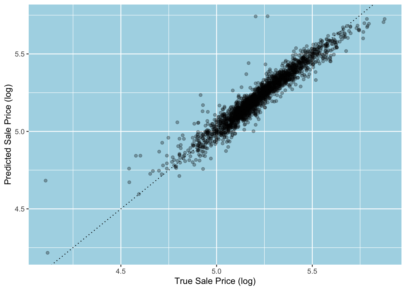
#> [1,] 0.05071922

Let’s have a look at the fit. We can use broom’s augment() function, which also accepts workflow objects. In that case, it expects data for its new_data argument and augments the data with fitted values (as “.pred”), residuals (as “.resid”) and more.³¹ Below, we see that three points stand out by laying way above the 45-degree line, which tells us that the sale price of these houses is overpredicted by the model by a wide margin.³²

augment(lm_fit, new_data = ames_train) |>
  ggplot(aes(Sale_Price, .pred)) +
  geom_point(alpha = 0.3) +
  geom_abline(lty = 3) +
  labs(
    x = "True Sale Price (log)", 
    y = "Predicted Sale Price (log)"
  )

Training using resamples

Previously, we resampled the training data to create 10 analysis and 10 assessment sets. We can use the fit_resamples() function in the tune package to train the model 10 times. To make this exercise more meaningful, let’s compare three linear regression models by producing performance metrics for them using the 10-fold cross-validation resamples we have created before. Do the preprocessing steps we have used earlier make any difference compared with no preprocessing? What if we extend the recipe by adding another step involving interaction terms?

Instead of creating and training three different workflows separately, we can create a workflow set using the workflowset() function in the worklowsets package. The function expects two main arguments: preproc, a list of recipes, and models, a list of model specifications.

Let’s create the recipes first. Since the baseline specification involves no preprocessing, we will use a formula instead of a recipe.³³ The third recipe extends the second recipe by including the step_interact() function to add interaction terms to the model.³⁴ The second recipe will create dummies from the Bldg_Type variable by concatenating “Bldg_Type” and its level names by an _. We use the starts_with() helper function to select all those dummies. The colon is used to indicate that the variables on both sides of it are to be interacted. The tilde indicates that the interaction terms are added to the right-hand side of the formula.

ames_rec1 = Sale_Price ~ .

ames_rec2 = 
  recipe(Sale_Price ~ ., data = ames_train) |>
  step_nzv(all_predictors()) |>
  step_YeoJohnson(all_numeric_predictors()) |>
  step_other(Neighborhood, threshold = 0.01) |>
  step_dummy(all_nominal_predictors())

ames_rec3 = 
  ames_rec2 |>
  step_interact(~ Gr_Liv_Area:starts_with("Bldg_Type_"))

Recall that the workflow() function expects a recipe list and a model specification list. Below we first create the preproc list for recipes. We do the same for model specification within the workflow_set() function call to create a workflow set, which is a tibble workflow set object.

preproc = list(
  no_prep = ames_rec1,
  prep = ames_rec2,
  prep_int = ames_rec3
)
lm_models = workflow_set(preproc, models = list(linear_reg()))
lm_models
#> # A workflow set/tibble: 3 × 4
#>   wflow_id            info             option    result    
#>   <chr>               <list>           <list>    <list>    
#> 1 no_prep_linear_reg  <tibble [1 × 4]> <opts[0]> <list [0]>
#> 2 prep_linear_reg     <tibble [1 × 4]> <opts[0]> <list [0]>
#> 3 prep_int_linear_reg <tibble [1 × 4]> <opts[0]> <list [0]>

The function creates a tibble to store the workflows. The id column stores workflow ids created by combining the recipe name with the model specification function name. The result column is currently empty and it is filled out with fit results once the workflow set is trained.

The workflowsets package provides the workflow_map() function to fit each workflow using some fit function in a purrr-like fashion.³⁵ The fn argument is for specifying the fit function name.³⁶ The other two arguments are seed for setting a seed integer before each function execution and verbose logical for logging progress. The additional options it takes are passed on to the fit function. Below, we pipe the workflow set to the workflow_map() function and pass in fn = "fit_resamples" to use the fit_resamples() function and resamples = ames_folds to provide cross-validation resamples to that function.

lm_results = lm_models |>
  workflow_map(
    # Options to `workflow_map()`:
    fn = "fit_resamples",
    seed = 143,
    verbose = TRUE,
    # Options to `fit_resamples()`:
    resamples = ames_folds
  )

lm_results workflow set now contains the fit results. The plus inside <> indicates that training was performed successfully. Since we have 10 cross-validation resamples, 10 fits were performed for each workflow.

lm_results
#> # A workflow set/tibble: 3 × 4
#>   wflow_id            info             option    result   
#>   <chr>               <list>           <list>    <list>   
#> 1 no_prep_linear_reg  <tibble [1 × 4]> <opts[1]> <rsmp[+]>
#> 2 prep_linear_reg     <tibble [1 × 4]> <opts[1]> <rsmp[+]>
#> 3 prep_int_linear_reg <tibble [1 × 4]> <opts[1]> <rsmp[+]>

We can use the collect_metrics() function to collect the performance metrics for each workflow and for each combination of workflows and resamples. The former returns the simple average of all performance metrics (10 in our case) for each workflow and we pass in summarize = TRUE to the function to do so. By default, two metrics are computed for the regression mode: root mean squared error (“rmse”) and r-squared (“rsq”).³⁷ Below, we collect only the mean RMSE for each workflow.

collect_metrics(lm_results, summarize = TRUE) |>
  filter(.metric == "rmse")
#> # A tibble: 3 × 9
#>   wflow_id         .config preproc model .metric .estimator   mean     n std_err
#>   <chr>            <chr>   <chr>   <chr> <chr>   <chr>       <dbl> <int>   <dbl>
#> 1 no_prep_linear_… Prepro… formula line… rmse    standard   0.0824    10 0.00606
#> 2 prep_linear_reg  Prepro… recipe  line… rmse    standard   0.0679    10 0.00374
#> 3 prep_int_linear… Prepro… recipe  line… rmse    standard   0.0683    10 0.00379

The first set of preprocessing steps helps to improve the model performance while adding interaction terms increases the prediction error.³⁸ We have evidence to select the second model as the best model. We now fit it to the entire training set and compute the test set RMSE using rmse() function from the yardstick package in tidymodels.³⁹

lm_final_wflow = 
  workflow() |>
  add_recipe(ames_rec2) |>
  add_model(linear_reg())

lm_final_fit = fit(lm_final_wflow, ames_train)

lm_final_fit |>
  augment(ames_test) |>
  rmse(truth = Sale_Price, estimate = .pred)
#> Warning in predict.lm(object = object$fit, newdata = new_data, type =
#> "response", : prediction from rank-deficient fit; consider predict(.,
#> rankdeficient="NA")
#> # A tibble: 1 × 3
#>   .metric .estimator .estimate
#>   <chr>   <chr>          <dbl>
#> 1 rmse    standard      0.0577

Finally, we select 20 of the statistically significant coefficients. We observe that houses with larger above-ground living areas tended to sell for higher prices. More recently built homes, properties in better overall condition, and those with larger garages also fetched higher prices. Among similar houses in all other respects, those in the Stone Brook neighborhood commanded the highest sale prices. An irregular lot shape and location in a commercial zone resulted in lower sale prices.

tidy(lm_final_fit) |>
  arrange(p.value) |>
  filter(p.value < 0.05) |>
  slice_head(n = 20)
#> # A tibble: 20 × 5
#>    term                                   estimate std.error statistic  p.value
#>    <chr>                                     <dbl>     <dbl>     <dbl>    <dbl>
#>  1 Gr_Liv_Area                             0.225    0.0180       12.5  1.24e-34
#>  2 Overall_Cond_Excellent                  0.261    0.0258       10.1  1.88e-23
#>  3 Overall_Cond_Good                       0.226    0.0238        9.48 6.61e-21
#>  4 Overall_Cond_Very_Good                  0.230    0.0243        9.46 7.73e-21
#>  5 Neighborhood_Stone_Brook                0.108    0.0120        9.01 4.38e-19
#>  6 Year_Built                              0.00119  0.000139      8.55 2.21e-17
#>  7 Overall_Cond_Above_Average              0.201    0.0237        8.46 4.77e-17
#>  8 Overall_Cond_Average                    0.187    0.0236        7.93 3.45e-15
#>  9 Neighborhood_Northridge_Heights         0.0852   0.0118        7.20 8.43e-13
#> 10 Sale_Condition_Normal                   0.0348   0.00507       6.86 8.73e-12
#> 11 Lot_Area                                0.00597  0.000932      6.41 1.79e-10
#> 12 Overall_Cond_Below_Average              0.148    0.0241        6.16 8.47e-10
#> 13 MS_SubClass_Duplex_All_Styles_and_Ages -0.0586   0.00967      -6.07 1.54e- 9
#> 14 Sale_Condition_AdjLand                  0.113    0.0199        5.69 1.45e- 8
#> 15 Neighborhood_Northridge                 0.0662   0.0126        5.27 1.53e- 7
#> 16 Lot_Shape_Irregular                    -0.0939   0.0181       -5.19 2.36e- 7
#> 17 Fireplaces                              0.0241   0.00476       5.05 4.67e- 7
#> 18 MS_Zoning_C_all                        -0.0954   0.0195       -4.90 1.05e- 6
#> 19 Overall_Cond_Fair                       0.121    0.0251        4.80 1.70e- 6
#> 20 Garage_Cars                             0.0155   0.00327       4.76 2.09e- 6

Summary

In this post, we used the tidymodels packages to perform some of the key tasks involved in a scheme of model training: data splitting and resampling (rsample), preprocessing (recipes) and model specification (parsnip), combining preprocessing with model specification to create workflows (workflows), and training a workflow and workflow sets (workflowsets). In the next post, we will explore the tidymodels packages further, particularly tune and dials, to see how we can tune model hyperparameters by focusing on tree-based models.

Footnotes

A lightweight introduction to tidymodels can be found on its official website. For an extensive exposition, see Kuhn and Silge (2023). See Boehmke and Greenwell (2020) for an in-depth exposition of supervised and unsupervised machine learning in R. Hastie et al. (2021) provide a very accessible explanation of main statistical learning methods and illustrate them in R and Python.↩︎
I thank Osman Can İçöz for his generous feedback on the draft version of this post. The usual disclamier applies.↩︎
For a description of the original data, see its documentation. The original data set has 82 columns. The modeldata version does not include a few quality columns that appear to be outcomes rather than predictors and has 74 columns in total. For other differences, see https://www.tmwr.org/ames.↩︎
In a typical regression exercise where inference is the primary objective, outliers will lead to large residuals violating the assumption of normality of residuals and yielding a large standard error. This will reduce the power of statistical tests for the coefficients. Plus, the log transformation ensures that predicted house prices are positive.↩︎
This is so because the Ames data set was already processed out of the raw data to eliminate any missing values. Typically, in any data set, there would be at least some columns with some missing values. In that case, one would want to know more than the total number of missing values. The visdat package provides the vis_miss() function to represent the missing data visually. Try running visdat::vis_miss(ames, cluster = TRUE).↩︎
Run class(ames_split) to see its class(es). Run typeof(ames_split) to view its type, which is a list.↩︎
For classification variables, random sampling is done in a way that the proportion of the event of interest is the same across the sets.↩︎
The Monte-Carlo cross-validation is a variant of cross-validation where a fixed proportion of data is randomly selected for the assessment set in each iteration in that the assessment sets are not mutually exclusive as in the regular cross-validation. rsample’s mc_cv() conducts this variant of cross-validation.↩︎
The default parameter values are 10 and 1, respectively. The function also has a strata argument to perform stratified random sampling.↩︎
ames_folds is both a vfold_split and rsplit object. Run class(ames_folds) to see this.↩︎
For time series data, resampling has to respect the sequential nature of the data. rsample’s rolling_origin() function performs rolling forecasting origin resampling by doing so.↩︎
Preprocessing is also known as feature engineering.↩︎
The term_info tibble, another element of ames_rec list, has the same structure as the var_info tibble. Until a recipe is processed by the prep() function, var_info and term_info contain the same variable names as the formula. We will get to the prep() function shortly.↩︎
This function requires two conditions to be met for near zero variance: 1) the predictor has very few unique values relative to the number of samples (by default, below 10%) and 2) the ratio of the frequency of the most common value to the frequency of the second most common value is large (by default, above 19 = 95/5)↩︎
step_nzv() and step_zv(), which removes zero variance variables, work with both numeric and categorical variables.↩︎
The steps and the variables they apply to are stored in the steps list of the ames_rec list.↩︎
For more on these transformations, see Boehmke and Greenwell (2020). Both transformations are parametric, driving the input variable towards normality by selecting the best parameter value to achieve this.↩︎
This function accepts numeric variables as well.↩︎
The downside is that such dummies will only take on zero in the training set and have zero variance. The corresponding coefficients in the linear regression case cannot be estimated; they will be “NA”.↩︎
The step_*() functions also accept starts_with(), matches(), etc. to help with variable selection.↩︎
Run class(ames_prep) and inspect ames_rec and ames_prep objects in your IDE to see this.↩︎
The function expects a trained recipe.↩︎
We need to put only the function name between quotation marks so no parentheses.↩︎
In the next post of the series, we will explore these arguments further.↩︎
For the full list of model specification functions offerred by parsnip, see https://www.tidymodels.org/find/parsnip/. We will cover some of them in this series.↩︎
If there is no preprocessing involved, the add_formula() function can be used instead of add_recipe() to pass in a formula to the workflow() function.↩︎
This is to say that lm_fit is a list workflow object, not a list of workflows. We will get to the workflow sets shortly.↩︎
See the section on feature engineering above on why this might be the case.↩︎
For instance, the variable MS_SubClass contains “Duplex_All_Styles_and_Ages” as a value, which essentially means that the dwelling is a duplex building. The variable Bldg_Type contains “Duplex” as a value to indicate the same fact. So when the dummies are created from these variables, the dummies corresponding to these values perfectly correlate with each other: if a property is duplex, both take on 1 and 0 otherwise. There are other similar cases, and the exact perfect colinearities depend on the random splits.↩︎
extract_fit_parsnip() also extracts the model fit but stores in an extended format.↩︎
When the underlying lm fit object is provided, it uses “.fitted” for fitted values and “..y” for the dependent variable.↩︎
The reference to the “rank-deficient fit” in the warning message has to do with the fact that lm() was not able to estimate some coefficients due to the reasons we outlined above. We can still predict, though.↩︎
You can use a regular recipe too, but you would need to add step_dummy(all_nominal_predictors()) to make sure prediction with test set observations works.↩︎
We do not use the standardization step in the recipes simply because this linear transformation of variables won’t help with the fit in the linear regression setting. It will only lead to different coefficient estimates.↩︎
In other words, it maps from the untrained workflow set to the trained workflow set using a specified fit/training function.↩︎
Its default value is “tune_grid”. We will explore this function further in the next post.↩︎
We can control the metrics. We will get to this in the next post of the series.↩︎
While it is already clear which model performs the best in this instance, the most proper way to make such a comparison involves some statistical test using the resampled performance metrics. I skip this step. For more on this topic, see Kuhn and Silge (2023).↩︎
We will say more on this package in the next post.↩︎